6.1 Aim

This chapter introduces the reader to the concepts involved in understanding the electrostatics which is relevant to radiographic science. This involves the consideration of electrical charge, charge distribution and electrical potential and potential difference.

6.2 Introduction

Electrostatics, as the name implies, is the study of static electrical charges. We are familiar with many examples of electrostatics from our ordinary lives, from sparks which may occur from our clothes when undressing, to the large discharges of electricity which occur during lightning strikes. Much of the early experimentation with electricity involved electrostatics. It was discovered at an early stage that there were two types of electrical charge, one called negative and the other positive. While it is mathematically convenient to regard charge in this way, it does not explain what electrical charge actually is and how it behaves. This will be the subject of this chapter.

6.3 Properties of electrical charges

The general properties of electrical charges are as follows:

• Charges can be considered as being of two types: positive and negative.

• The smallest unit of negative charge which can exist in isolation is that possessed by an electron, and the smallest unit of positive charge which can exist in isolation is that possessed by a proton.

• Electrical charges exert forces on each other even when they are separated by a vacuum. The forces are mutual, equal and opposite, as expected by Newton’s third law (see Sect. 3.5).

• Like charges (i.e. charges of the same sign) repel each other while unlike charges (of opposite signs) attract each other.

  Page 34 

• The magnitude of the mutual forces between the charges is influenced by:

the magnitude of the individual charges

the medium in which they are embedded, being greatest when the medium is a vacuum

the inverse square of the distance between the charged bodies – this is another application of the inverse square law (see Ch. 26).

• Electrical charges may be induced in a body by the proximity of a charged body, leading to a force of attraction between the two bodies.

• Electrical charges may flow easily in some materials (called electrical conductors) and with difficulty in other materials (called electrical insulators). Both types of material are capable of having charges induced in them.

• When electrical charges move, they produce a magnetic field.

6.4 Force between two electrical charges in a vacuum

Consider two charges, q₁ and q₂, separated by a distance, d, in a vacuum, as shown in Figure 6.1.

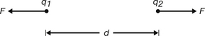
Figure 6.1 The forces (F) between two electrical charges, q₁ and q₂, separated by a distance (d) are equal and opposite.

If we assume that both charges are of the same sign, then q₁ will exert a force of repulsion (F) on q₂ and q₂ will exert the same force of repulsion on q₁. As we have already stated above, it can be shown that:

Thus, F is proportional to the magnitude of each charge and to the inverse square of the distance separating them.

If we combine the factors in 1, 2 and 3 above, we can produce the equation:

Equation 6.1

If q₁ and q₂ both have the same sign, then F will be positive and will represent a force of repulsion. If the charges have opposite signs, then F will be negative and will represent a force of attraction.

If we wish to replace the proportionality sign in Equation 6.1 by an equals sign then we need to introduce a constant of proportionality (see Appendix A). This equation now reads:

Equation 6.2

This equation is often referred to as Coulomb’s law of force between two charges and has particular relevance when we consider the charges between subatomic particles (see Chs 18 and 19).

The constant of proportionality is , where ε₀ is the permittivity of a vacuum and has a value of 6.85 × 10⁻¹² F.m⁻¹. The charges q₁, and q₂ are expressed in coulombs, the separation d is in meters and the force F is in newtons.

The coulomb corresponds to the charge carried by 6 × 10¹⁸ electrons or protons. An alternative (and more practical) definition of the coulomb is:

Insight

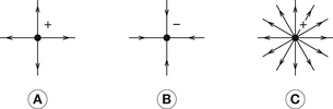
The influence of the inverse square law on the force between charged bodies may be grasped if we assume that charged bodies emanate lines of force in all direction similar to the light emission from a point source of light obeying the inverse square law. The number of such lines is proportional to the magnitude of the charge (analogous to the brightness of the light source). This is shown diagrammatically in Figure 6.2, where the arrows point in the direction of force experienced by a positive charge if placed at that point. There will be further discussion of lines of force in the section of this chapter dealing with electrical field strength (see Sect. 6.6).

Figure 6.2 Electric ‘lines of force’ associated with (A) a weak positive charge, (B) a weak negative charge and (C) a strong positive charge.

6.5 Permittivity and relative permittivity (dielectric constant)

Equation 6.2 only holds true when the charges are in a vacuum, as ε₀ is the permittivity of a vacuum. In any other medium, the equation requires to be modified to:

Equation 6.3

where ε is the permittivity of the medium.

It is, however, often convenient to compare the permittivity of the medium relative to that of a vacuum, e.g. if the permittivity of the medium is twice that of a vacuum, then the relative permittivity (K) is 2. This can be obtained from the simple formula:

or by cross-multiplying:

Equation 6.4

so Equation 6.3 may be rewritten as:

Equation 6.5

K is known as the dielectric constant of the medium and so we can see that the relative permittivity and the dielectric constant are the same. Note that as the dielectric constant is a comparative number, it does not have any units. (The dielectric constant is further discussed in Ch. 13 where we consider its importance in capacitors.)

6.6 Electrical field strength

We have already seen that an electrical charge is capable of influencing other charges placed at a distance from it. This influence on other charges at a distance is known as a field and, for the purpose of comparing electrical charges, E is measured in units of newton/coulomb. Consider the electrical field around a point charge. If we wish to know the field strength at a point, we simply place a unit of positive charge at that point and measure the magnitude and direction of the force exerted upon it. If we consider Equation 6.5 and have q₂=1 (unit charge), then we can say:

Equation 6.6

We have already considered a diagrammatic representation of a field around a point charge (Fig. 6.2). The arrows represent the direction of the force acting on a unit positive charge (if placed at that point) and the line density represents the intensity of the electrical field.

6.7 Electrostatic induction of charge

As mentioned earlier (Sect 6.3), a charge may be induced on an electrical conductor or on an insulator. Each will now be considered.

6.7.1 Induction of a conductor

The situation that exists if an electrically charged body (B) is placed close to a conductor (A) is shown in Figure 6.3. A conductor is a body which will allow a flow of electrons. The positive charge on B attracts electrons to it and leaves equal numbers of positive charges on the opposite surface of A. Notice that the opposite charge is induced on the surface of the conductor closest to the inducing charge and that equal numbers of positive and negative charges are induced. Eventually a state of equilibrium is reached where the electrons on the surface of A experience an equal force of attraction from the two sets of positive charge. When this happens, no further electron flow takes place.

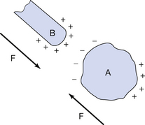
Figure 6.3 Induction of a charge on a conducting body, A, results in a force of attraction, F, with the inducing body, B.

The charge distribution results in a net force of attraction as the unlike charges are closer to the charged body than the like charges.

Withdrawal of the charged body results in uniform distribution of the charges in A.

6.7.2 Induction of an insulator (dielectric)

If we bring a charged body close to an insulator, a similar force of attraction occurs – this can be demonstrated by running a comb through your hair and holding it close to a small piece of paper, which will be attracted to it. This result is somewhat surprising, as electrons cannot move as freely through an insulator as a conductor. Some insulators are more efficient at producing induced charges than others and it is found that this varies with the dielectric constant (see Sect. 6.5) of the material. There are two explanations of the induced charge in an insulator, molecular distortion and polar molecules.

6.7.2.1 Molecular distortion

A body is composed of atoms or molecules. These contain equal numbers of protons (+ve) and electrons (−ve), thus making the body electrically neutral. As can be seen in Figure 6.4A, the electrons normally form symmetrical orbits around the nucleus so that the average position of the electron is over the nucleus, and the two sets of charges cancel each other out. If a charged body is placed close to the atom (Fig. 6.4B), the electron orbits are distorted relative to the atomic nucleus. The average position of the electrons is now displaced to one side of the atom, and so the atom has been polarized into an electrical dipole.

Figure 6.4 The effect of an external field on an atom. (A) The atom with no external field applied; (B) the polarization of the atom to form a dipole caused by the proximity of a negatively charged body.

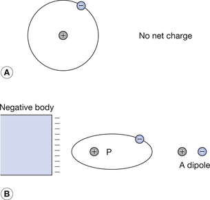
6.7.2.2 Polar molecules

Some molecules exist in which the atoms are so arranged that the average position of the electrons is not coincident with that of the nuclei, even when the atoms are not subject to an electrical field. These molecules are polarized even when not subject to an electrical field.

The effect of an external electric field is to rotate these molecules such that they tend to become aligned with the field. This means that the structure now has definite positive and negative ends. Adjacent dipoles cancel each other’s effects. Practical dielectrics use such materials as they produce a much stronger effect than molecular distortion alone.

6.8 Electrical potential

There are a number of similarities between electrical potential and potential energy. In the case of potential energy, this represents the work done raising a body to a height from a zero level. Similar concepts will now be discussed for electrical potential.

6.8.4 Electrical potential due to a point charge

Consider a point charge, Q, as shown in Figure 6.5. A unit of positive charge has been moved from infinity to a distance r from Q. The nearer the charge comes to Q, the greater the force of repulsion (if Q is positive) or attraction (if Q is negative). Thus the potential is positive if Q is positive and negative if Q is negative since the potential is the work done on the unit positive charge. If we consider that the work done on all unit positive charges which are equidistant from Q will be the same, then it is logical to assume that equipotential surfaces will be concentric spheres with Q as the centre. It is also worth noting that the particular path chosen to bring a unit positive charge from infinity to the point r is of no importance and so paths (1) and (2) give exactly the same electrical potential.

Figure 6.5 The electrical potential energy of a point charge, Q.

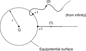
Electrical potential is usually given the symbol V and so we can produce the equation:

Equation 6.8

where V is in volts, Q is in coulombs and r is in metres.

The electrical potential due to a point charge is given the term coulomb potential and the force between two charges is the coulomb force (see Sect. 6.4).

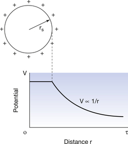
6.8.5 Electrical potential due to a conducting sphere

If we place a charge Q on a conducting sphere, then the charged particles will mutually repel each other and the charges will be evenly distributed on the outer surface of the sphere as shown in Figure 6.5. This is true whether the sphere is hollow or solid. No potential difference exists between any points either on the surface or within the sphere (if a potential difference did exist, the charge would redistribute in such a way that the whole body was at a constant potential). When the potential exists outside the sphere, it may be shown mathematically that the sphere behaves as though all the charge Q is placed at its centre. This is shown in the graph in Figure 6.6 (See page 38). Thus Equation 6.8 can be used to calculate the potential of points outside the sphere where r is the distance from the centre of the sphere. This is important from a practical viewpoint in radiography in the design of components such as the X-ray tube shield where we wish to have the charge distributed evenly over the internal surfaces of the tube shield.

Figure 6.6 Distribution of electrical potential on a conducting sphere of radius r. The potential is constant within the sphere and reduces outside it (V ∝ 1/r).

6.9 Distribution of electrical charge on an irregulary shaped conductor

Having considered the charge distribution on a sphere, it is now useful to consider the distribution of charge on a conducting body of irregular shape. Such a body is shown in Figure 6.7. Again the charge is distributed so that no potential difference exists between any points within the body. This gives the charge distribution shown in Figure 6.7. Note that there are large collections of charge at parts of the body that have a small radius of curvature. This is important in the design of the X-ray tube both in the prevention of coronal discharge (where electrons are forcibly removed from their orbits to create an electrical spark) from sharp corners and also the use of a sharp-edged focusing cup for electron focusing (see Ch. 30).

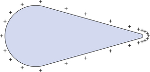
Figure 6.7 Distribution of positive charge on an irregularly shaped conductor. Note the high intensity of charge at the area of low radius of curvature.