Measurement Concepts
Measurement is the process of assigning “numbers to objects (or events or situations) in accord with some rule” (Kaplan, 1963, p. 177). The numbers assigned can indicate numerical values or categories. Instrumentation, a component of measurement, is the application of specific rules to develop a measurement device (instrument). Instrumentation produces trustworthy evidence that we can use to evaluate the outcomes of research.
The rules of measurement ensure that values or categories are assigned consistently from one subject (or event) to another and, eventually, if the measurement strategy is found to be meaningful, from one study to another. The rules of measurement established for research are similar to those used in nursing practice. For example, when nurses measure the urine output from patients, they use an accurate measurement container, observe the amount of urine in the container in a consistent way, and precisely record the urine output on the chart. This practice ensures accuracy and precision and reduces the amount of error. When one is measuring the abdominal girth to detect changes in ascites, the skin on the abdomen is marked to ensure that the measurement is always taken the same distance below the waist. With this method, any change in measurement can be attributed to a change in ascites rather than an inadvertent change in the measurement site. Developing accurate and precise measures of concepts important to nursing practice is a major focus of nursing research.
It is important for researchers to understand the logic within measurement theory so they can select, use, and develop quality measurement methods for their studies. As with most theories, measurement theory uses terms with meanings that can be best understood within the context of the theory. The following explanation of the logic of measurement theory includes definitions of directness of measurement, measurement error, levels of measurement, reference of measurement, reliability, validity, accuracy, precision, sensitivity, specificity, and likelihood ratio. The chapter concludes with a discussion of the process for appraising validity in qualitative research.
DIRECTNESS OF MEASUREMENT
Measurement begins by clarifying the object, characteristic, or element to be measured. Only then can one identify or develop strategies or methods to measure it. In some cases, identification of the measurement object and measurement strategies can be simple and straightforward, as when we are measuring concrete factors, such as a person’s height or wrist circumference; this is referred to as direct measurement. Health care technology has made direct measures of concrete elements—such as height, weight, temperature, time, space, movement, heart rate, and respiration—familiar to us. Technology is also available to measure many bodily functions and biological and chemical characteristics. The focus of measurement theory in these instances is in the accuracy and precision of the measurement method. Nurses are also experienced in gathering direct measures of attribute or demographic variables, such as age, gender, ethnic origin, diagnosis, marital status, income, and education.
Often in nursing, however, the characteristic we want to measure is an abstract idea, such as pain, stress, depression, anxiety, caring, or coping. If the element to be measured is abstract, it is best clarified through a conceptual definition. We can then use the conceptual definition to select or develop appropriate means of measuring the concept. The instrument or measurement strategy used in the study must match the conceptual definition. An abstract concept is not measured directly; instead, indicators or attributes of the concept are used to represent the abstraction. This is referred to as indirect measurement. For example, indicators of coping skills might be the frequency or accuracy of identifying the problem, the creativity in selecting solutions, and the speed or effectiveness in resolving the problem. Rarely, if ever, can a single measurement strategy completely examine or measure all the aspects of an abstract concept.
MEASUREMENT ERROR
There is no perfect measure. Error is inherent in any measurement strategy. Measurement error is the difference between what exists in reality and what a research instrument measures. Measurement error exists in both direct and indirect measures and can be random or systematic. Direct measures, which are considered to be highly accurate, are subject to error. For example, the scale may not be accurate, laboratory equipment may be precisely calibrated but may change with use, or the tape measure may not be placed in the same location or held at the same tension for each measurement.
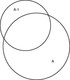
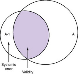
There is also error in indirect measures. Efforts to measure concepts usually result in measuring only part of the concept or measures that identify an aspect of the concept but also contain other elements that are not part of the concept. Figure 15-1 shows a Venn diagram of the concept A measured by instrument A-1. As the figure shows, A-1 does not measure all of A. In addition, some of what A-1 measures is outside the concept of A. Both of these situations are examples of errors in measurement.
Types of Measurement Errors
Two types of errors are of concern in measurement: random error and systematic error. To understand these types of errors, we must first understand the elements of a score on an instrument or an observation. According to measurement theory, there are three components to a measurement score: the true score (T), the observed score (O), and the error score (E). The true score is what we would obtain if there was no error in measurement. Because there is always some measurement error, the true score is never known. The observed score is the measure obtained. The error score is the amount of random error in the measurement process. The theoretical equation of these three measures is as follows:

This equation is a means of conceptualizing random error and not a basis for calculating it. Because the true score is never known, the random error is never known, only estimated. Theoretically, the smaller the error score, the more closely the observed score reflects the true score. Therefore, using measurement strategies that reduce the error score improves the accuracy of the measurement.
A number of factors can occur during the measurement process that increase random error. They are (1) transient personal factors, such as fatigue, hunger, attention span, health, mood, mental set, and motivation; (2) situational factors, such as a hot stuffy room, distractions, the presence of significant others, rapport with the researcher, and the playfulness or seriousness of the situation; (3) variations in the administration of the measurement procedure, such as interviews in which wording or sequence of questions is varied, questions are added or deleted, or researchers code responses differently; and (4) processing of data, such as errors in coding, accidentally marking the wrong column, punching the wrong key when entering data into the computer, or incorrectly totaling instrument scores.
Random error causes individuals’ observed scores to vary haphazardly around their true score. For example, with random error, one subject’s observed score may be higher than his or her true score, whereas another subject’s observed score may be lower than his or her true score. According to measurement theory, the sum of random errors is expected to be zero, and the random error score (E) is not expected to correlate with the true score (T). Thus, random error does not influence the direction of the mean but, rather, increases the amount of unexplained variance around the mean. When this occurs, estimation of the true score is less precise.
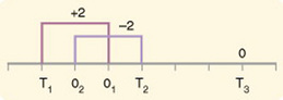
If you were to measure a variable for three subjects and diagram the random error, it might appear as shown in Figure 15-2. The difference between the true score of subject 1 (T1) and the observed score (O1) is two positive measurement intervals. The difference between the true score (T2) and observed score (O2) for subject 2 is two negative measurement intervals. The difference between the true score (T3) and observed score (O3) for subject 3 is zero. The random error for these three subjects is zero (+2 - 2 + 0 = 0). In viewing this example, one must remember that this is only a means of conceptualizing random error.
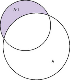
Measurement error that is not random is referred to as systematic error. A scale that weighed subjects 2 pounds more than their true weights demonstrates systematic error. All of the body weights would be higher, and, as a result, the mean would be higher than it should be. Systematic error occurs because something else is being measured in addition to the concept. A conceptualization of systematic error is presented in Figure 15-3. Systematic error (represented by shaded area in the figure) is due to the part of A-1 that is outside of A. This part of A-1 measures factors other than A and will bias scores in a particular direction.
Systematic error is considered part of T (true score) and reflects the true measure of A-1, not A. Adding the true score (with systematic error) to the random error (which is 0) yields the observed score, as shown by the following equations:
You will incur some systematic error in almost any measure; however, a close link between the abstract theoretical concept and the development of the instrument can greatly decrease systematic error. Because of the importance of this factor in a study, researchers spend considerable time and effort refining their measurement instruments to decrease systematic error.
Another effective means of diminishing systematic error is to use more than one measure of an attribute or a concept and to compare the measures. To make this comparison, researchers use a variety of data collection methods, such as interview and observation. Campbell and Fiske (1959) developed a technique of using more than one method to measure a concept, referred to as the multimethod-multitrait technique. More recently, the technique has been described as a version of methodological triangulation, as discussed in Chapter 10. These techniques allow researchers to measure more dimensions of the abstract concept, and the effect of the systematic error on the composite observed score decreases. Figure 15-4 illustrates how more dimensions of concept A are measured through the use of four instruments, designated A-1, A-2, A-3, and A-4.
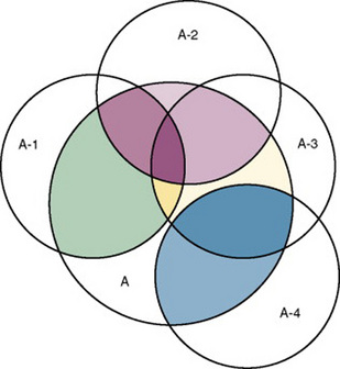
For example, a researcher could decrease systematic error in measures of anxiety by (1) administering Taylor’s Manifest Anxiety Scale, (2) recording blood pressure readings, (3) asking the subject about anxious feelings, and (4) observing the subject’s behavior. Multimethod techniques decrease systematic error by combining the values in some way to give a single observed score of anxiety for each subject. Sometimes, however, it may be difficult logically to justify combining scores from various measures, and triangulation may be the most appropriate approach. Using triangulation, the researcher decreases systematic error by performing a series of bivariate (two variable) correlations on the matrix of values.
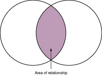
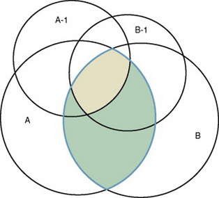
In some studies, researchers use instruments to examine relationships. Consider a hypothesis that tests the relationship between concept A and concept B. In Figure 15-5, the shaded area enclosed in the dark lines represents the true relationship between concepts A and B. If two instruments (A-1 and B-1) are used to examine the relationship between concepts A and B, the part of the true relationship actually reflected by these measures is represented by light colored areas in Figure 15-6. Because two instruments provide a more accurate measure of concepts A and B, more of the true relationship between concepts A and B can be measured.
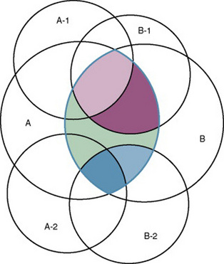
If additional instruments (A-2 and B-2) are used to measure concepts A and B, more of the true relationship might be reflected. Figure 15-7 demonstrates the parts of the true relationship with four colors that might be reflected if two instruments are used to measure concept A (A-1 and A-2) and two instruments to measure concept B (B-1 and B-2).
LEVELS OF MEASUREMENT
The traditional levels of measurement have been used for so long that the categorization system has been considered absolute and inviolate. In 1946, Stevens organized the rules for assigning numbers to objects so that a hierarchy in measurement was established. The levels of measurement, from lower to higher, are nominal, ordinal, interval, and ratio.
Nominal-Scale Measurement
Nominal-scale measurement is the lowest of the four measurement categories. It is used when data can be organized into categories of a defined property but the categories cannot be ordered. For example, ethnicity is nominal data with categories such as African American, Caucasian, or Hispanic. One cannot say that one category is higher than another or that category A (African American) is closer to category B (Caucasian) than to category C (Hispanic). The categories differ in quality but not quantity. Therefore, one cannot say that subject A possesses more of the property being categorized than does subject B. (Rule: The categories must be unorderable.) Categories must be established so that each datum will fit into only one of the categories. (Rule: The categories must be exclusive.) All the data must fit into the established categories. (Rule: The categories must be exhaustive.) Data such as gender, marital status, and diagnoses are examples of nominal data. When data are coded for entry into the computer, the categories are assigned numbers. For example, gender may be classified as 1 = male, 2 = female. The numbers assigned to categories in nominal measurement are used only as labels and cannot be used for mathematical calculations.
Ordinal-Scale Measurement
Data that can be measured at the ordinal-scale level can be assigned to categories of an attribute that can be ranked. There are rules for how one ranks data. As with nominal-scale data, the categories must be exclusive and exhaustive. With ordinal-scale data, the quantity of the attribute possessed can be identified. However, it cannot be demonstrated that the intervals between the ranked categories are equal. Therefore, ordinal data are considered to have unequal intervals. Scales with unequal intervals are sometimes referred to as ordered metric scales.
Many scales used in nursing research are ordinal levels of measure. For example, one could rank intensity of pain, degrees of coping, levels of mobility, ability to provide self-care, or daily amount of exercise on an ordinal scale. For daily exercise, the scale could be 0 = no exercise; 1 = moderate exercise, no sweating; 2 = exercise to the point of sweating; 3 = strenuous exercise with sweating for at least 30 minutes per day; 4 = strenuous exercise with sweating for at least 1 hour per day. This type of scale may be referred to as a metric ordinal scale.
Interval-Scale Measurement
In interval-scale measurement, distances between intervals of the scale are numerically equal. Such measurements also follow the previously mentioned rules: mutually exclusive categories, exhaustive categories, and rank ordering. Interval scales are assumed to be a continuum of values. Thus, the researcher can identify the magnitude of the attribute much more precisely. However, it is not possible to provide the absolute amount of the attribute because of the absence of a zero point on the interval scale.
Fahrenheit and centigrade temperatures are commonly used as examples of interval scales. A difference between a temperature of 70 °F and one of 80 °F is the same as the difference between a temperature of 30 °F and one of 40 °F. We can measure changes in temperature precisely. However, it is not possible to say that a temperature of 0 °C means the absence of temperature.
Ratio-Level Measurement
Ratio-level measurements are the highest form of measure and meet all the rules of the lower forms of measures: mutually exclusive categories, exhaustive categories, rank ordering, equal spacing between intervals, and a continuum of values. In addition, ratio-level measures have absolute zero points. Weight, length, and volume are common examples of ratio scales. Each has an absolute zero point, at which a value of zero indicates the absence of the property being measured: Zero weight means the absence of weight. In addition, because of the absolute zero point, one can justifiably say that object A weighs twice as much as object B, or that container A holds three times as much as container B. Laboratory values are also an example of ratio level of measurement where the individual with a fasting blood sugar (FBS) of 180 has an FBS twice that of an individual with a normal FBS of 90. To help expand your understanding of levels of measurement (nominal, ordinal, interval, and ratio) and to apply this knowledge, Grove (2007) developed a statistical workbook focused on examining the levels of measurement, sampling methods, and statistical results in published studies.
The Importance of Level of Measurement for Statistical Analyses
An important rule of measurement is that one should use the highest level of measurement possible. For example, you can collect data on age (measured) in a variety of ways: (1) you can obtain the actual age of each subject (ratio level of measurement); (2) you can ask subjects to indicate their age by selecting from a group of categories, such as 20 to 29, 30 to 39, and so on (ordinal level of measurement); or (3) you can use a bivariate measure such as under 65 and over 65 (nominal level of measurement). The highest level of measurement in this case is the actual age of each subject. If you need age categories for specific analyses in your research, the computer can be instructed to establish them from the initial age data.
The level of measurement is associated with the types of statistical analyses that can be performed on the data. Mathematical operations are limited in the lower levels of measurement. With nominal levels of measurement, only summary statistics, such as frequencies, percentages, and contingency correlation procedures, can be used. In the age example, however, you can perform more sophisticated analyses if you have obtained the actual age of each subject. The age variable is measured at the ratio level (actual age of the subject) so the data can be entered into the computer and analyzed with stronger statistical techniques. Variables measured at the interval or ratio level can be analyzed with the strongest statistical techniques available.
Controversy over Measurement Levels
In recent years, controversy has erupted over justification for the system used to categorize measurement levels, dividing researchers into two factions: the fundamentalists and the pragmatists. Pragmatists regard measurement as occurring on a continuum rather than by discrete categories, whereas fundamentalists adhere rigidly to the original system of categorization.
The primary focus of the controversy relates to the practice of classifying data into the categories ordinal and interval. The controversy developed because, according to the fundamentalists, many of the current statistical analysis techniques can be used only with interval data. Many pragmatists believe that if researchers rigidly adhered to Stevens’s rules, few if any measures in the social sciences would meet the criteria to be considered interval-level data. They also believe that violating Stevens’s criteria does not lead to serious consequences for the outcomes of data analysis. Thus, pragmatists often treat ordinal data as interval data, using statistical methods to analyze them such as the t-test and analysis of variance (ANOVA), which are traditionally reserved for interval or ratio level data. Fundamentalists insist that the analysis of ordinal data be limited to statistical procedures designed for ordinal data, such as nonparametric procedures.
There is also a controversy about the statistical operations that can justifiably be performed with scores from the various levels of measure (Armstrong, 1981, 1984; Knapp, 1984, 1990). For example, can one calculate a mean using ordinal data? Fundamentalists believe that appropriate statistical analysis is contingent on the level of measurement. They disagree with the contention that the scaling procedures used for most psychosocial instruments provide interval-level data. This is related to scale definition, which we discuss in Chapter 16.
For example, the Likert scale uses the scale points “strongly disagree,” “disagree,” “uncertain,” “agree,” and “strongly agree.” Numerical values (e.g., 1, 2, 3, 4, and 5, respectively) are assigned to these categories. Fundamentalists claim that equal intervals do not exist between these categories. It is not possible to prove that there is the same magnitude of feeling between “uncertain” and “agree” as there is between “agree” and “strongly agree.” Therefore, they hold, parametric analyses cannot be used. Pragmatists believe that with many measures taken at the ordinal level, such as scaling procedures, an underlying interval continuum is present that justifies the use of parametric statistics.
Our position is more like that of the pragmatists than of the fundamentalists. Many nurse researchers analyze data from Likert scales as though the data were interval level. However, some of the data in nursing research are obtained through the use of crude measurement methods that can be classified only into the lower levels of measurement. Therefore, we have included the nonparametric statistical procedures needed for their analysis in the statistical chapters.
REFERENCE TESTING OF MEASUREMENT
Referencing involves comparing a subject’s score against a standard. Two types of testing involve referencing: norm-referenced testing and criterion- referenced testing. Norm-referenced testing addresses the question “How does the average person score on this test?” It involves the use of standardization that has been developed over several years, with extensive reliability and validity data available. Standardization involves collecting data from thousands of subjects expected to have a broad range of scores on the instrument. From these scores, population parameters such as the mean and standard deviation (described in Chapter 19) can be developed. Evidence of the reliability and validity of the instrument can also be evaluated through the use of the methods described later in this chapter. The best-known norm-referenced test is the Minnesota Multiphasic Personality Inventory (MMPI), which is used commonly in psychology and occasionally in nursing research.
Criterion-referenced testing asks the question “What is desirable in the perfect subject?” It involves comparing a subject’s score with a criterion of achievement that includes the definition of target behaviors. When the subject has mastered these behaviors, he or she is considered proficient in the behavior. The criterion might be a level of knowledge or desirable patient outcome measures. Criterion measures are not as useful in research as they might be in evaluation studies or evaluation of clinical expertise. Faculty use criterion measures to evaluate student performance in clinical agencies. For example, a clinical evaluation form would include the critical behaviors the student is expected to master in a pediatric course to be clinically competent to care for pediatric patients at the end of the course.
RELIABILITY
The reliability of a measure denotes the consistency of measures obtained in the use of a particular instrument and indicates the extent of random error in the measurement method. For example, if the same measurement scale is administered to the same individuals at two different times, the measurement is reliable if the individuals’ responses to the items remain the same (assuming that nothing has occurred to change their responses). For example, if you measure oral temperatures of 10 individuals every 5 minutes 10 times using the same thermometer for all measures of all individuals, and at each measurement the individuals’ temperatures change, being sometimes higher than before and sometimes lower, you begin to question the reliability of the thermometer. If two data collectors observe the same event and record their observations on a carefully designed data collection instrument, the measurement would be reliable if the recordings from the two data collectors are comparable. The equivalence of their results would indicate the reliability of the measurement technique. If responses vary each time a measure is performed, there is a chance that the instrument is not reliable—that is, that it yields data with a large random error.
Reliability plays an important role in the selection of scales for use in a study. Researchers need instruments that are reliable and provide values with only a small amount of random error. Reliable instruments enhance the power of a study to detect significant differences or relationships actually occurring in the population under study. Therefore, it is important to test the reliability of an instrument before using it in a study. Estimates of reliability are specific to the sample being tested. Thus, high reported reliability values on an established instrument do not guarantee that its reliability will be satisfactory in another sample or with a different population. Therefore, you must perform reliability testing on each instrument used in your study before you perform other statistical analyses. The reliability values must be included in published reports of the study.
Reliability testing examines the amount of random error in the measurement technique. It is concerned with characteristics such as dependability, consistency, precision, and comparability. Because all measurement techniques contain some random error, reliability exists in degrees and is usually expressed as a form of correlation coefficient, with 1.00 indicating perfect reliability and 0.00 indicating no reliability. A reliability coefficient of 0.80 is considered the lowest acceptable value for a well-developed psychosocial measurement instrument. The coefficient of 0.80 (or 80%) indicates the instrument is 80% reliable with 20% random error (Grove, 2007). For a newly developed psychosocial instrument, a reliability coefficient of 0.70 is considered acceptable as the researcher refines the instrument to achieve a reliability of 0.80. Higher levels of reliability (0.90 to 0.99) are essential for physiological measures that are used to determine “critical” physiological functions such as cardiac output. Reliability testing focuses on the following three aspects of reliability: stability, equivalence, and homogeneity.
Stability
Stability is concerned with the consistency of repeated measures of the same attribute with the use of the same scale or instrument over time. It is usually referred to as test-retest reliability. This measure of reliability is generally used with physical measures, technological measures, and paper-and-pencil scales. The technique requires an assumption that the factor to be measured remains the same at the two testing times and that any change in the value or score is a consequence of random error.
Physical measures and equipment can be tested and then immediately retested, or the equipment can be used for a time and then retested to determine the necessary frequency of recalibration. For example, the diagnosis of osteoporosis is made by bone mineral density (BMD) study of the hip, spine, and wrist. The BMD score is determined with the dual-energy x-ray absorptiometry (DEXA or DXA) scan. Because the BMD does not change rapidly in people even with treatment, the test-retest over a week time period should demonstrate reliable or consistent DXA scan scores for patients.
With paper-and-pencil measures, a period of 2 weeks to 1 month is recommended between the two testing times. After retesting, the investigator performs a correlational analysis on the scores from the two measures. A high correlation coefficient indicates high stability of measurement by the instrument. Test-retest reliability has not proved to be as effective with paper-and-pencil measures as originally anticipated. The procedure presents a number of problems. Subjects may remember their responses at the first testing time, leading to overestimation of the reliability. Subjects may actually be changed by the first testing and therefore may respond to the second test differently, leading to underestimation of the reliability.
Test-retest reliability requires the assumption that the factor being measured has not changed between the measurement points. Many of the phenomena studied in nursing, such as hope, coping, and anxiety, do change over short intervals. Thus, the assumption that if the instrument is reliable, values will not change between the two measurement periods may not be justifiable. If the factor being measured does change, the test is not a measure of reliability. In fact, if the measures stay the same even though the factor being measured actually has changed, the instrument may lack reliability.
Equivalence
Equivalence compares two versions of the same paper-and-pencil instrument or two observers measuring the same event. Comparison of two observers is referred to as interrater reliability. Comparison of two paper-and-pencil instruments is referred to as alternate-forms reliability or parallel-forms reliability. Alternative forms of instruments are of more concern in the development of normative knowledge testing. When repeated measures are part of the design, however, alternative forms of measurement, although not commonly used, would improve the design. Demonstrating that one is actually testing the same content in both tests is extremely complex, and thus, the procedure is rarely used in clinical research.
Determining interrater reliability is a more immediate concern in research and is used in many observational studies. Interrater reliability values must be reported in any study in which observational data are collected or judgments are made by two or more data gatherers. Two techniques determine interrater reliability. Both techniques require that two or more raters independently observe and record the same event using the protocol developed for the study or that the same rater observes and records an event on two occasions. To adequately judge interrater reliability, the raters must observe at least 10 subjects or events (Washington & Moss, 1988). A DVD can be used to record the same event on two occasions. Every data collector used in the study must be tested for interrater reliability.
The first procedure for calculating interrater reliability requires a simple computation involving a comparison of the agreements obtained between raters on the coding form with the number of possible agreements. This calculation is performed through the use of the following equation:
This formula tends to overestimate reliability, a particularly serious problem if the rating requires only a dichotomous judgment. In this case, there is a 50% probability that the raters will agree on a particular item through chance alone. Appropriate correlational techniques can be used to provide a more accurate estimate of interrater reliability. If more than two raters are involved, a statistical procedure to calculate coefficient alpha (discussed later in this chapter) may be used. ANOVA may also be used to test for differences among raters. There is no absolute value below which interrater reliability is unacceptable. However, any value below 0.80 should generate serious concern about the reliability of the data or of the data gatherer (or both). The interrater reliability value is best to be 0.90, which means 90% reliability and 10% random error. The process for determining interrater reliability and the value achieved must be included in research reports.
When raters know they are being watched, their accuracy and consistency are considerably better than when they believe they are not being watched. Thus, interrater reliability declines (sometimes dramatically) when the raters are assessed covertly (Topf, 1988). You can develop strategies to monitor and reduce the decline in interrater reliability, but they may entail considerable time and expense.
The coding of data into categories, which is a frequent step done in qualitative research, has received little attention in regard to reliability. Two types of reliability are related to categorizing data: unitizing reliability and interpretive reliability. Unitizing reliability assesses the extent to which each judge (data collector, coder, researcher) consistently identifies the same units within the data as appropriate for coding. This is of concern in observational studies and studies using text transcribed from interviews. In observational studies, the data collector must select particular units of what is being observed as appropriate to record and code. Of concern is the extent to which two data collectors observing the same event would select the same units to record. In studies using transcribed text from interviews, the researcher must select particular units of the transcribed text to code into preselected categories. To what extent would two individuals reading the same text select the same passages to code into categories (Garvin, Kennedy, & Cissna, 1988)?
In some studies, the selection of units for coding is simple and straightforward. For example, a unit may begin when a person starts talking. In other studies, however, the identification of an appropriate unit for coding may require some level of inference or judgment on the part of the rater. For example, if the unit began when the baby awakened, the rater would have to determine at what point the baby was indeed awake. Studies in which every event in the unit is coded require less inference than studies in which only select acts in the unit are to be coded. In all cases, reliability improves when the researcher clearly identifies the units to be coded rather than relying on the judgment of the coder (Marshall & Rossman, 2006; Washington & Moss, 1988). Guetzkow’s (1950) index (U) can be used to calculate unitizing reliability (Garvin et al., 1988).
Interpretive reliability assesses the extent to which each judge assigns the same category to a given unit of data. Most studies using categories report only a global level of reliability in which the overall rate of reliability is examined. The most commonly used measure of global reliability is Guetzkow’s (1950) P, which reports the extent to which the judges agree in the selection of categories. A more desirable method of calculating the extent of agreement between judges is Cohen’s (1960) Kappa statistic. However, global measures of interpretive reliability provide no information on the degree of consistency in assigning data to a particular category. Category-by-category measures of reliability include the assumption that some categories are more difficult to use than others and thus have a lower reliability. To use this method of evaluating reliability, you must (1) statistically analyze the reliability category by category, (2) determine the equality of the frequency distribution among categories, and (3) examine the possibility that coders may be systematically confusing some categories (Garvin et al., 1988).
Homogeneity
Tests of instrument homogeneity, used primarily with paper-and-pencil tests, address the correlation of various items within the instrument. The original approach to determining homogeneity was split-half reliability. This strategy was a way of obtaining test-retest reliability without administering the test twice. Rather, the instrument items were split in odd-even or first-last halves, and a correlational procedure was performed between the two halves. Researchers have generally used the Spearman-Brown correlation formula for this procedure. One of the problems with the procedure was that although items were usually split into odd-even items, it was possible to split them in a variety of ways. Each approach to splitting the items would yield a different reliability coefficient. Therefore, the researcher could continue to split the items in various ways until a satisfactorily high coefficient was obtained.
More recently, testing the homogeneity of all the items in the instrument has been seen as a better approach to determining reliability. Although the mathematics of the procedure are complex, the logic is simple. One way to view it is as though one conducted split-half reliabilities in all the ways possible and then averaged the scores to obtain one reliability score. Homogeneity testing examines the extent to which all the items in the instrument consistently measure the construct. It is a test of internal consistency. The statistical procedures used for this process are Cronbach’s alpha coefficient for interval and ratio level data and, when the data are dichotomous, the Kuder-Richardson formula (K-R 20).
If the Cronbach’s alpha coefficient value were 1.00, each item in the instrument would be measuring exactly the same thing. When this occurs, one might question the need for more than one item. A slightly lower coefficient (0.8 to 0.9) indicates an instrument that will reflect more richly the fine discriminations in levels of the construct. Magnitude of the instrument reliability can then be discerned more clearly. Bakas, Champion, Perkins, Farran, and Williams (2006) conducted a psychometric study to test the revised 15-item Bakas Caregiving Outcomes Scale (BCOS) and provided the following internal consistency and test-retest reliability data to support the 15-item BCOS reliability.
The original 10-item BCOS was improved by adding five items addressing financial well-being, level of energy, role functioning, physical functioning, and general health [resulting in the 15-item BCOS]. (p. 346)
 INTERNAL CONSISTENCY RELIABILITY AND TEST-RETEST RELIABILITY
Internal consistency reliability for the 15-item BCOS was supported by a Cronbach’s alpha of 0.90 (n = 147); the 10-item BCOS had an alpha = 0.85. A small subsample (n = 36) also completed the BCOS 2 weeks later, with Cronbach’s alpha of 0.81 for the 15-item BCOS and .75 for the 10-item BCOS. The ICC [intraclass correlation coefficient] assessing 2-week test-retest reliability were 0.66 for the 15-item BCOS and 0.68 for the 10-item BCOS. (Bakas et al., 2006, p. 350; full-text article available in CINAHL)
Other approaches to testing internal consistency are (1) Cohen’s Kappa statistic, which determines the percentage of agreement with the probability of chance being taken out; (2) correlating each item with the total score for the instrument; and (3) correlating each item with each other item in the instrument. This procedure, often used in instrument development, allows researchers to identify items that are not highly correlated and delete them from the instrument. Factor analysis may also be used to develop instrument reliability. The number of factors being measured influences the instrument’s reliability and total scores may be more reliable than subscores in determining reliability. After performing the factor analysis, the researcher can delete instrument items with low factor weights. After these items have been deleted, reliability scores on the instrument will be higher. For instruments with more than one factor, correlations can be performed between items and factor scores. Estok, Sedlak, Doheny, and Hall (2007) conducted a study to develop a structural model for osteoporosis preventing behaviors in postmenopausal women and one of the scales they used was the Osteoporosis Self-Efficacy Scale (OSES). The researchers documented the reliability of this scale by providing internal consistency reliability (Cronbach alpha) for the total scale and subscales (identified through factor analysis) for previous studies and the current study.
It is essential that an instrument be both reliable and valid for measuring a study variable in a population. If the instrument has low reliability values, then it cannot be valid because its measurement is inconsistent. An instrument that is reliable cannot be assumed to be valid for a particular study or population. Thus, you will need to determine the validity of the instrument you are using for your study, which you can accomplish in a variety of ways.
VALIDITY
The validity of an instrument determines the extent to which it actually reflects the abstract construct being examined. Validity has been discussed in the literature in terms of three primary types: content validity, predictive validity, and construct validity. Within each of these types, subtypes have been identified. These multiple types of validity were very confusing, especially because the types were not discrete but interrelated.
Currently, validity is considered a single broad method of measurement evaluation that is referred to as construct validity and includes content and predictive validity (Berk, 1990; Rew, Stuppy, & Becker, 1988). All of the previously identified types of validity are now considered evidence of construct validity. In 1985, in its Standards for Educational and Psychological Testing, the American Psychological Association (APA) published standards used to judge the evidence of validity. This important work greatly extends our understanding of what validity is and how to achieve it. According to the APA, validity addresses the appropriateness, meaningfulness, and usefulness of the specific inferences made from instrument scores. It is important to note that it is the inferences made from the scores, not the scores themselves, that are important to validate (Goodwin & Goodwin, 1991).
Validity, like reliability, is not an all-or-nothing phenomenon but, rather, a matter of degree. No instrument is completely valid. Thus, one determines a measure’s degree of validity rather than whether or not it has validity. Defining the validity of an instrument requires years of work. Many equate the validity of the instrument with the rigorousness of the researcher. The assumption is that because the researcher develops the instrument, the researcher also develops the validity. However, this is to some extent an erroneous assumption, as Brinberg and McGrath (1985) have pointed out.
Figure 15-8 illustrates validity (the shaded area) by the extent to which the instrument A-1 reflects concept A. As measurement of the concept improves, validity improves. The extent to which the instrument A-1 measures items other than the concept is referred to as systematic error (also identified as the unshaded area of A-1 in Figure 15-8). As systematic error decreases, validity increases.
Validity varies from one sample to another and from one situation to another; therefore, validity testing actually validates the use of an instrument for a specific group or purpose rather than the instrument itself. An instrument may be valid in one situation but not valid in another. Therefore, validity should be reexamined in each study situation, but this often does not happen.
Because many instruments used in nursing studies were developed for use in other disciplines, it is important that any measure chosen for a nursing study be valid in terms of nursing knowledge. Nagley and Byers (1987) provided an example of a study in which a measure of cognitive function was used to gauge confusion. However, the instrument did not capture the nursing meaning of confusion. Nurses consider persons confused who do not know their age or location. The aforementioned measure of cognitive function does not categorize such persons as confused.
Content-Related Validity Evidence
Content-related validity evidence examines the extent to which the method of measurement includes all the major elements relevant to the construct being measured. This evidence is obtained from the following three sources: the literature, representatives of the relevant populations, and content experts.
In the 1970s, the only type of validity that most studies addressed was referred to as face validity, which verified basically that the instrument looked like it was valid or gave the appearance of measuring the content it was suppose to measure. This approach is no longer considered acceptable evidence for validity. However, it is still an important aspect of the usefulness of the instrument, because the willingness of subjects to complete the instrument relates to their perception that the instrument measures the content they agreed to provide (Lynn, 1986; Thomas, Hathaway, & Arheart, 1992).
Documentation of content-related validity evidence begins with development of the instrument. The first step of instrument development is to identify what is to be measured; this is referred to as the universe or domain of the construct. You can determine your domain through a concept analysis or an extensive literature search. Qualitative methods can also be used for this purpose. Johnson and Rogers (2006) developed the Medication-Taking Questionnaire based on purposeful action dimensions to determine individuals’ decision-making process for adherence to medication treatment for hypertension. They described their initial instrument development process as follows.
You must describe the procedures used to develop or select items for the instrument that represent the domain of the construct. One helpful strategy commonly used is to develop a blueprint or matrix, such as is used in developing test items for an examination. However, before developing such items, the blueprint specifications must be submitted to an expert panel to validate that they are appropriate, accurate, and representative. At least five experts are recommended, although a minimum of three experts is acceptable if you cannot locate additional individuals with expertise in the area (Lynn, 1986). You might seek out individuals with expertise in various fields, for example, one with knowledge of instrument development, a second with clinical expertise in an appropriate field of practice, and a third with expertise in another discipline relevant to the content area.
Give the experts specific guidelines for judging the appropriateness, accuracy, and representativeness of the specifications. Berk (1990) recommended that the experts first make independent assessments and then meet for a group discussion of the specifications. You can then revise the specifications and resubmit them to the experts for a final independent assessment. Davis (1992) recommended that the researcher provide expert reviewers with theoretical definitions of concepts and a list of which instrument items are expected to measure each of the concepts. Ask the reviewers to judge how well each of the concepts has been represented in the instrument.
You then need to determine how to measure the domain. The item format, item content, and procedures for generating items must be carefully described. Items are then constructed for each cell in the matrix, or observational methods are designated to gather data related to a specific cell. You will be expected to describe the specifications used in constructing items or selecting observations. Sources of content for items must be documented. Then you can assemble, refine, and arrange the items in a suitable order before submitting them to the content experts for evaluation. Specific instructions for evaluating each item and the total instrument must be given to the experts.
Use the content validity index (CVI) developed by Waltz and Bausell (1981) to obtain a numerical value that reflects the level of content-related validity evidence. With this instrument, experts rate the content relevance of each item using a 4-point rating scale. Lynn (1986, p. 384) recommended standardizing the options on this scale to read as follows: “1 = not relevant; 2 = unable to assess relevance without item revision or item is in need of such revision that it would no longer be relevant; 3 = relevant but needs minor alteration; 4 = very relevant and succinct.” In addition to evaluating existing items, ask the experts to identify important areas not included in the instrument. As presented earlier, Johnson and Rogers (2006) developed the Medication-Taking Questionnaire (MTQ): Purposeful Action and described their content validity testing process and outcomes as follows.
Content validity testing was undertaken to determine clarity and relevance of content. Participants and experts were given verbal instructions and a packet consisting of a consent form, written instructions, clarity instrument, content validity instrument, and demographic questionnaire. The clarity instrument asked participants to rate items as clear or unclear (Imle & Atwood, 1988). Participants were given a definition of each subscale and asked to rate each item’s relevancy using a 4-point scale from 1 (irrelevant) to 4 (extremely relevant; Lynn, 1986). Space was provided to make comments after each rating procedure. (p. 339)
Items met clarity criterion if 70% of participants rated the item as clear and the content validity criterion if 80% of participants rated the item as 3 or 4 (Imle & Atwood, 1988; Lynn, 1986). The comments from the clarity and content validity criterion were used to revise the MTQ: Purposeful Action items and subscales…
Of the 20 MTQ: Purpose Action items, 19 achieved clarity and content validity agreement. The 1 item that had an unacceptable clarity agreement was eventually eliminated from the questionnaire. Professionals expressed a concern about the lack of specificity in the questions, but that was not an issue for the hypertensive participants. For example, one professional indicated that the item, “Blood pressure pills keep me from having problems,” lacked specificity. Because the purpose of this questionnaire was to establish a general screening tool for individuals who potentially may choose not to take their medications rather than to create a diagnostic tool, the participants’ scores were given priority. Of the 20 items [see Table 15-1 for the 20 items in the original questionnaire], 12 underwent minor grammatical revisions guided by the comments of both the participants and professionals. For example, items were made specific to blood pressure and the term medication was changed to pills. Several items were reworded, or the tense of the verb was changed. (Johnson & Rogers, 2006, pp. 341–342)
TABLE 15-1
Medication-Taking Questionnaire: Purposeful Action Initial 20 Items Statistics
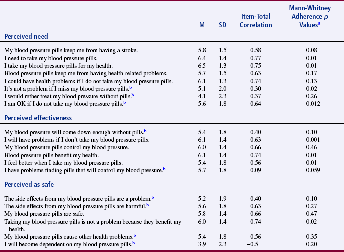
aDifference between low (scored 1–3) versus high (scored 7–10) adherence.
bReverse coded.
From Johnson, M. J., & Rogers, S. (2006). Development of the Purposeful Action Medication-Taking Questionnaire. Western Journal of Nursing Research, 28(3), 344.
Before sending the instrument to experts for evaluation, decide how many experts must agree on each item and on the total instrument in order for the content to be considered valid. Items that do not achieve minimum agreement by the expert panel must be either eliminated from the instrument or revised. Johnson and Rogers (2006) described their panel of reviewers, who were health professionals and patients prescribed antihypertensive medications, for their MTQ: Purposeful Action MTQ in the following except.
Johnson and Rogers (2006) provided excellent detail about the development of their questionnaire and the process for determining content validity. They also provided extensive information about the expert review panel for conducting the content validity testing. The strength of the review panel is that it included both health professionals and patients taking medications for hypertension. The MTQ: Purposeful Action was a Likert scale with 7-point response options (described earlier), so it would be clearer if the researchers had called the MTQ a scale versus a questionnaire.
With some modifications, this procedure can also be used with existing instruments, many of which have never been evaluated for content-related validity. With the permission of the author or researcher who developed the instrument, you could revise the instrument to improve its content-related validity (Lynn, 1986). In addition, Berk (1990) has suggested that the panel of experts or judges asked to evaluate the instrument items for content validity also examine it in terms of readability and the possibility that its language might offend subjects or data gatherers.
Readability of an Instrument
Readability is an essential element of the validity and reliability of an instrument. Assessing an instrument’s level of readability is relatively simple and takes about 20 minutes. There are more than 30 readability formulas. These formulas count language elements in the document. They then use this information to estimate the degree of difficulty a reader may have in comprehending the text. Readability formulas are now a standard part of word-processing software. Table 15-2 provides instructions for using the Fog formula to determine the readability of a measurement method.
TABLE 15-2
How to Find the Fog Index (Fog Formula)
1. Pick a sample of writing 100 to 125 words long. Count the average number of words per sentence. In counting, treat independent clauses as separate sentences. “In school we studied; we learned; we improved” is three sentences.
2. Count the words of three syllables or more. Do not count: (a) capitalized words, (b) combinations of short words such as butterfly or manpower, or (c) verbs made into three syllables by adding “–es” or “–ed” such as trespasses or created. Divide the count of long words by the number of words in the passage to get the percentage.
3. Add the results from no. 1 (average sentence length) and no. 2 (percentage of long words). Multiply the sum by 0.4. Ignore the numbers after the decimal point.
4. The result is the years of schooling needed to easily understand the passage tested. Few readers have more than 17 years of schooling, so give any passage higher than 17 a Fog Index of 17-plus.
Adapted from Gunning, R., & Kallan, R. A. (1994). How to take the fog out of business writing. Chicago: Dartnell. The Fog IndexSM is a service mark licensed exclusively to RK Communication Consultants by D. and M. Mueller.
Although readability has never been formally identified as a component of content validity, it should be. How valid is content that is incomprehensible? Miller and Bodie (1994) suggested that the researcher should directly assess the reading comprehension level of the study population before using a formula to calculate an instrument’s readability. They indicated that it is a mistake to assume that someone’s literacy is equivalent to the last grade level the individual completed. They recommended that researchers use the Classroom Reading Inventory (CRI), which is based on the Flesch, Space, Dale, and Fry reading comprehension scales (Silvaroli, 1986). This instrument determines the level at which an individual can comprehend written material without assistance. Johnson and Rogers (2006) described the readability of their MTQ: Purposeful Action as follows.
Evidence of Validity from Factor Analysis
Exploratory factor analysis can be performed to examine relationships among the various items of the instrument. Items that are closely related are clustered into a factor. The analysis may reveal the presence of several factors, which may indicate that the instrument reflects several constructs rather than a single construct. The researcher can validate the number of constructs in the instrument and measurement equivalence among comparison groups through the use of confirmatory factor analysis (Goodwin & Goodwin, 1991; Stommel, Wang, Given, & Given, 1992; Teel & Verran, 1991). Items that do not fall into a factor (and thus do not correlate with other items) may be deleted. We further describe validity from factor analysis in Chapter 20.
Johnson and Rogers (2006) conducted an exploratory factor analysis (EFA) to determine the factor structure for their MTQ: Purposeful Action. The EFA identifies the specific factors or subscales for the scale and the items that fit each of these subscales. The original scale had 20 items sorted into three subscales (labeled perceived need, perceived effectiveness, and perceived as safe) that were identified in Table 15-1. The EFA and the results are described as follows:
Factor analysis is a grouping technique that allows for evaluation of the dimensionality of scales (Munro, 2001; Nunnally & Bernstein, 1994). A principle axis factoring solution with an oblimen rotation, considered the best analysis for achieving a theoretical solution uncontaminated by unique and random error variability was undertaken….
The EFA yielded two interpretable factors [see Table 15-3], which eliminated six additional items because of factor loadings < 0.40. The first factor merged the need and effectiveness items along with one item from the Safe subscale. This factor was renamed treatment benefits (benefits). The second factor, renamed medication safety (safety), was reduced to three of the original safe subscales items.
TABLE 15-3
Principal Axis Factor Analysis with Oblimen Rotation Pattern (and Structure in Parentheses) Coefficients for the MTQ: Purposeful Action Two-Factor Solution
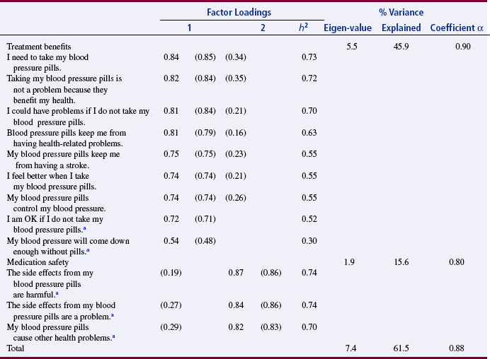
aItem required reverse coding. Factor loadings in parenthesis represent structure coefficients. If patterned or structure coefficient is not listed, the value was < 0.15.
From Johnson, M. J., & Rogers, S. (2006). Development of the Purposeful Action Medication-Taking Questionnaire. Western Journal of Nursing Research, 28(3), 345.
The Benefits subscale retained nine items that focused on the actual perceived benefits of treatment, such as preventing a stroke, controlling blood pressure, preventing further health problems, and feeling better when taking medications, which indicated a desire to control blood pressure to maintain and promote health and well-being. The subscale had an eigenvalue of 5.5 and a total item variance explained by the factor of 46%.…
The Safety subscale (three items) focused on side effects of medications. This subscale had an eigenvalue of 1.9 and a total item variance explained by the factor of 16%…Together, the two factor solution had a coefficient alpha [Cronbach alpha] of 0.87 and an explained variance of 62%. (Johnson & Rogers, 2006, pp. 343–346)
Johnson and Rogers (2006) initially developed a 20-item scale with three subscales (see Table 15-1). Based on the content validity testing and the EFA, the scale was reduced from 20 to 12 items that were organized into two subscales (treatment benefit and medication safety) (see Table 15-3). These researchers provide an excellent rationale for the revisions that they made in their MTQ: Purposeful Action. In this study, the revised scale demonstrated homogeneity reliability (Cronbach alpha = 0.87) and construct validity through content validity testing and EFA. Johnson and Rogers (2006, p. 348) also conducted confirmatory factor analysis that “supported the hypothesis that benefits and safety underlie the cognitive component of medication taking in hypertensive medications.”
Evidence of Validity from Structural Analysis
Structural analysis is now being used to examine the structure of relationships among the various items of an instrument. This approach provides insights beyond that provided by factor analysis. Factor analysis determines what items group together. Structural analysis determines how each item is related to other items. Thus, structural analysis goes a step beyond factor analysis. The exact relationship of each item in a factor is examined through correlational analyses.
Evidence of Validity from Contrasting (or Known) Groups
To test the instrument’s validity, identify groups that are expected (or known) to have contrasting scores on the instrument. Generate hypotheses about the expected response of each of these known groups to the construct. Next, select samples from at least two groups that are expected to have opposing responses to the items in the instrument. Hagerty and Patusky (1995) developed a measure called the Sense of Belonging Instrument (SOBI). They tested the instrument on the following three groups: community college students, clients diagnosed with major depression, and retired Roman Catholic nuns, as described in the following excerpt.
The nuns had the highest sense of belonging, the student groups followed, and the depressed group had the lowest sense of belonging. This test increased the validity of the instrument in that the scores of groups were as anticipated.
Evidence of Validity from Examining Convergence
In many cases, several instruments are available to measure a construct, for example, depression. But, for a number of possible reasons, the existing instruments may not be satisfactory for a particular purpose or a particular population. Therefore, the researcher may choose to develop a new instrument for a study. In examining the validity of the new instrument, it is important to determine how closely the existing instruments measure the same construct as the newly developed instrument (convergent validity). Administer all of the instruments (the new one and the existing ones) to a sample concurrently, and then evaluate the results using correlational analyses. If the measures are highly positively correlated, the validity of each instrument is strengthened. Johnson and Rogers (2006) strengthened the validity of their 12-item MTQ: Purposeful Action and its subscales (benefit and safety) by correlating them with a variety of other instruments (Hamilton Health Belief Model Hypertension [HBM] Scale with the HBM subscales of Susceptibility, Severity, Benefits, and Barriers; Lifestyle Busyness Questionnaire with Busyness and Routine subscales; and Blood Pressure Feedback Log). The results of these correlations are presented in Table 15-4. The significant positive correlations of 0.3 to 0.63 between the existing scales (Hamilton HBM Scale with Susceptibility and Benefits subscales and the Blood Pressure Feedback Log for adherent group) and the MTQ and the benefits subscale add to the construct validity of these instruments. This is an example of evidence of validity from examining convergence, which was strong for the MTQ and the benefit subscale but not the safety subscale.
TABLE 15-4
Validity Correlation Coefficients for the MTQ: Purposeful Action and Subscales
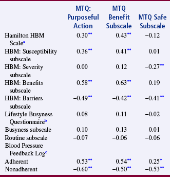
Note: HBM is the Health Belief Model Hypertension Scale.
an = 107.
bn = 104.
cn = 102.
*p < 0.05, two-tailed.
**p < 0.01, two-tailed.
From Johnson, M. J., & Rogers, S. (2006). Development of the Purposeful Action Medication-Taking Questionnaire. Western Journal of Nursing Research, 28(3), 346.
Evidence of Validity from Examining Divergence
Sometimes, instruments can be located that measure a construct opposite to the construct measured by the newly developed instrument (divergent validity). For example, if the newly developed instrument measures hope, you and your research team could search for an instrument that measures despair. If possible, you could administer this instrument and the instruments used to test convergent validity at the same time. You will perform correlational procedures with all the measures of the construct. If the divergent measure negatively correlates with other measures, validity for each of the instruments is strengthened. Johnson and Rogers (2006) also obtained evidence of validity from examining divergence for their MTQ: Purposeful Action. In Table 15-4, you will note that the MTQ and the subscales benefits and safety were significantly, negatively correlated with HBM Barriers subscale and the Blood Pressure Feedback Log for nonadherent hypertensive patients. These scales measure the opposite construct from the MTQ and its subscales, so these significant negative correlations indicated that the construct validity was strengthened for these instruments.
Evidence of Validity from Discriminant Analysis
Sometimes, instruments have been developed to measure constructs closely related to the construct measured by the newly developed instrument. If such instruments can be located, you can strengthen the validity of the two instruments by testing the extent to which the two instruments can finely discriminate between these related concepts. Testing of this discrimination involves administering the two instruments simultaneously to a sample and then performing a discriminant analysis. Chapter 21 discusses discriminant analysis.
Evidence of Validity from Prediction of Future Events
The ability to predict future performance or attitudes on the basis of instrument scores adds to an instrument’s validity. For example, nurse researchers might want to determine the ability of a scale that measures health-related behaviors to predict the future health status of individuals. One approach might be to examine reported stress levels of these individuals for the past 3 years. The validity of the Holmes and Rahe Life Events Scale, for example, could be tested in this manner. Miller (1981) discussed the validity and reliability of the Holmes and Rahe Life Events Scale in measuring stress levels in a variety of populations. The accuracy of predictive validity is determined through regression analysis.
Evidence of Validity from Prediction of Concurrent Events
Validity can be tested by examining the ability to predict the current value of one measure on the basis of the value obtained on the measure of another concept. For example, you might be able to predict the self-esteem score of an individual who had a high score on an instrument to measure coping. For example, a person who received a high score on coping might be expected to also have a high self-esteem score. If these results held true in a study in which both measures were obtained concurrently, the two instruments would have evidence of concurrent validity.
Successive Verification of Validity
After the initial development of an instrument, other researchers begin using the instrument in unrelated studies. Each of these studies adds to the validity information on the instrument. Thus, there is a successive verification of the validity of the instrument over time. For example, when additional researchers use the MTQ: Purposeful Action in their studies, this will add or subtract from the validity of this questionnaire.
ACCURACY AND PRECISION OF PHYSIOLOGICAL MEASURES
Accuracy and precision of physiological and biochemical measures tend not to be reported in published studies. These routine physiological measures are assumed to be accurate and precise, an assumption that is not always correct. The most common physiological measures used in nursing studies are blood pressure, heart rate, weight, and temperature. These measures are often obtained from the patient’s record with no consideration given to their accuracy. It is important to consider the possibility of differences between the obtained value and the true value of physiological measures. Thus, researchers using physiological measures must provide evidence of the accuracy of their measures (Gift & Soeken, 1988).
The evaluation of physiological measures may require a slightly different perspective from that applied to behavioral measures, in that standards for physiological measures are defined by the National Bureau of Standards rather than the APA. The construct by which physiological accuracy is judged consists of human physiology and the mechanics of physiological equipment. However, the process is similar to that used for behavioral measures and must be addressed. Gift and Soeken (1988) identified the following five terms as critical to the evaluation of physiological measures: accuracy, selectivity, precision, sensitivity, and error.
Accuracy
Accuracy is comparable to validity, in which evidence of content-related validity addresses the extent to which the instrument measured the domain defined in the study. For example, measures of pulse oximetry could be compared with arterial blood gas measures, and pulse oximetry should produce comparable values to blood gases to be considered an accurate measure. The researcher must be able to document the extent to which the measure is an effective predictive clinical instrument. For example, peak expiratory flow rate can predict asthma episodes.
Selectivity
Selectivity, an element of accuracy, is “the ability to identify correctly the signal under study and to distinguish it from other signals” (Gift & Soeken, 1988, p. 129). Because body systems interact, the researcher must choose instruments that have selectivity for the dimension being studied. For example, electrocardiographic readings allow one to differentiate electrical signals coming from the myocardium from similar signals coming from skeletal muscles.
To determine the content validity of biochemical measures, contact experts in the laboratory procedure and ask them to evaluate the procedure used for collection, analysis, and scoring. You might also ask them to judge the appropriateness of the measure for the construct being measured. Use contrasted groups’ techniques by selecting a group of subjects known to have high values on the biochemical measures and comparing them with a group of subjects known to have low values on the same measure. In addition, to obtain concurrent validity, compare the results of the test with results from the use of a known, valid method (DeKeyser & Pugh, 1990).
Precision
Precision is the degree of consistency or reproducibility of measurements made with physiological instruments. Precision is comparable to reliability. The precision of most physiological instruments is determined by the manufacturer and is part of quality control testing. Because of fluctuations in most physiological measures, test-retest reliability is inappropriate. Engstrom (1988, p. 389) stated that assessment of precision for physiological variables that yield continuous data must include “mean, minimal, and maximal differences; standard deviation of the net differences; technical error of measurement; and indices of agreement.” She suggested displaying these differences graphically and recommended exploratory data analysis (EDA) techniques for summarizing differences. Correlation coefficients are not adequate tests of the precision of physiological measures.
Two procedures are commonly used to determine the precision of biochemical measures. One is the Levy-Jennings chart. For each analysis method, a control sample is analyzed daily for 20 to 30 days. The control sample contains a known amount of the substance being tested. The mean, the standard deviation, and the known value of the sample are used to prepare a graph of the daily test results. Only 1 value of 22 is expected to be greater than or less than 2 standard deviations from the mean. If two or more values are more than 2 standard deviations from the mean, the method is unreliable in that laboratory. Another method of determining the precision of biochemical measures is the duplicate measurement method. The same technician performs duplicate measures on randomly selected specimens for a specific number of days. Results will be the same each day if there is perfect precision. Results are plotted on a graph, and the standard deviation is calculated on the basis of difference scores. The use of correlation coefficients is not recommended (DeKeyser & Pugh, 1990).
Sensitivity
Sensitivity of physiological measures relates to “the amount of change of a parameter that can be measured precisely” (Gift & Soeken, 1988, p. 130). If changes are expected to be small, the instrument must be very sensitive to detect the changes. Thus, sensitivity is associated with effect size (see Chapter 14). With some instruments, sensitivity may vary at the ends of the spectrum. This is referred to as the frequency response. The stability of the instrument is also related to sensitivity. This feature may be judged in terms of the ability of the system to resume a steady state after a disturbance in input. For electrical systems, this feature is referred to as freedom from drift (Gift & Soeken, 1988).
Error
Sources of error in physiological measures can be grouped into the following five categories: environment, user, subject, machine, and interpretation. The environment affects both the machine and the subject. Environmental factors include temperature, barometric pressure, and static electricity. User errors are caused by the person using the instrument and may be associated with variations by the same user, different users, changes in supplies, or procedures used to operate the equipment. Subject errors occur when the subject alters the machine or the machine alters the subject. In some cases, the machine may not be used to its full capacity. Machine error may be related to calibration or to the stability of the machine. Signals transmitted from the machine are also a source of error and can cause misinterpretation (Gift & Soeken, 1988).
Sources of error in biochemical measures are biological, preanalytical, analytical, and postanalytical. Biological variability in biochemical measures is due to factors such as age, gender, and body size. Variability in the same individual is due to factors such as diurnal rhythms, seasonal cycles, and aging. Preanalytical variability is due to errors in collecting and handling of specimens. These errors include sampling the wrong patients; using an incorrect container, preservative, or label; lysis of cells; and evaporation. Preanalytical variability may also be due to patient intake of food or drugs, exercise, or emotional stress. Analytical variability is associated with the method used for analysis and may be due to materials, equipment, procedures, and personnel used. The major source of postanalytical variability is transcription error. You can greatly reduce this source of error by entering data into the computer directly (DeKeyser & Pugh, 1990).
In Estok et al.’s (2007) study, introduced earlier in this chapter, the researchers used a dual-energy x-ray absorptiometry (DXA) scan to measure the bone mineral density (BMD) of their subjects. They provided a strong description of this physiological measurement device by discussing the accuracy, precision, and potential for error of the DXA. In addition, they described the scoring for the DXA scan, with the results being standardized using World Health Organization evidence-based guidelines for determining normal, osteopenia, and osteroporosis diagnoses. The DXA scan measurement method, the process for obtaining the BMD scores, and the meaning of the scores are described in the following excerpt:
USE OF SENSITIVITY, SPECIFICITY, AND LIKELIHOOD RATIOS TO DETERMINE THE QUALITY OF DIAGNOSTIC TESTS
An important part of evidence-based practice is the use of quality diagnostic tests to determine the presence or absence of disease. Clinicians want to know what laboratory or imaging study to order to help screen for or diagnose a disease. When you order a test, how can you be sure that the results are valid or accurate? The accuracy of a screening test or a test used to confirm a diagnosis is evaluated in terms of its ability to correctly assess the presence or absence of a disease or condition as compared to a gold standard. The gold standard is the most accurate means of currently diagnosing a particular disease and serves as a basis for comparison with newly developed diagnostic or screening tests. If the test is positive, what is the probability that the disease is present? If the test is negative, what is the probability that the disease is not present? When you talk to the patient about the results of their tests, how sure are you that they do or do not have the disease? Sensitivity and specificity are the terms used to describe the accuracy of a screening or diagnostic test (Table 15-5). There are four possible outcomes of a screening test for a disease: (1) true positive, which accurately identifies the presence of a disease; (2) false positive, which indicates a disease is present when it is not; (3) true negative, which indicates accurately that a disease is not present; or (4) false negative, which indicates that a disease is not present when it is (Grove, 2007). The 2 × 2 contingency table shown in Table 15-5 will help you to visualize sensitivity and specificity and these four outcomes (Melnyk & Fineout-Overholt, 2005).
TABLE 15-5
Results of Sensitivity and Specificity of Screening Tests
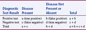
a = The number of people who have the disease and the test is positive (true positive).
b = The number of people who do not have the disease and the test is positive (false positive).
c = The number of people who have the disease and the test is negative (false negative).
d = The number of people who do not have the disease and the test is negative (true negative).
Grove, S. K. (2007). Statistics for health care research: A practical workbook. Philadelphia: Saunders, p. 335.
Sensitivity and specificity can be calculated based on research findings and clinical practice outcomes to determine the most accurate diagnostic or screening tool to use in identifying the presence or absence of a disease for a population of patients. The calculations for sensitivity and specificity are provided as follows:


Sensitivity is the proportion of patients with the disease who have a positive test result or true positive. The ways the researcher or clinician might refer to the test sensitivity include the following:
• Highly sensitive test is very good at identifying the diseased patient.
• If a test is highly sensitive, it has a low percentage of false negatives.
• Low sensitivity test is limited in identifying the patient with a disease.
• If a test has low sensitivity, it has a high percentage of false negatives.
• Therefore, if a sensitive test has negative results, the patient is less likely to have the disease.
• Use the acronym SnNout, which is read: High sensitivity (Sn), test is negative (N), rules the disease out (out).
Specificity of a screening or diagnostic test is the proportion of patients without the disease who have a negative test result or true negative. The ways the researcher or clinician might refer to the test specificity include the following:
• Highly specific test is very good at identifying the patients without a disease.
• If a test is very specific, it has a low percentage of false positives.
• Low specificity test is limited in identifying patients without disease.
• If a test has low specificity, it has a high percentage of false positives.
• Therefore, if a specific test has positive results the patient is more likely to have the disease.
• Use the acronym SpPin, which is read: High specificity (Sp), test is positive (P), rules the disease in (in).
Porter, Fleisher, Kohane, and Mandl (2003) conducted a prospective observational study to assess predictive value of parents reporting the medical history and physical signs of dehydration in their children. Their study included 132 parent-child dyads. The primary outcome was percentage of dehydration and secondary outcomes were clinically important acidosis and hospital admission. They also compared the reports of physical signs of dehydration made by the parents and the nurse. Their study results indicated that parent reports of physical symptoms and history had a higher sensitivity (range 73% to 100%) than specificity (range 0% to 49%) for predicting dehydration of 5% or greater in their child (Table 15-6). The nurse reports of physical signs for clinically important dehydration were always more specific (33% to 93%) than the parents (17% to 82%) and usually more sensitive (10% to 100%) than the parents (0% to 91%) (Table 15-7) (Porter et al., 2003). In this study, the nurses’ diagnostic ability to determine clinically important dehydration is the gold standard used as a basis for comparison of the parents’ diagnostic ability. As expected, the nurses’ were more sensitive and specific in diagnosing clinically important dehydration in children than were parents, but the parents were very sensitive in reporting the child’s history that predicated dehydration. In developing a diagnostic or screening test, researchers must achieve the highest sensitivity and specificity possible, and clinicians must select the most sensitive and specific screening test to diagnose diseases in their patients (Craig & Smyth, 2007; Grove, 2007). However, the screening test selected for detecting a disease is affected by cost as well as sensitivity and specificity.
TABLE 15-6
Value of Parent Reported History for Prediction of Clinically Important Dehydration
| Historical Element (Total No. of Parents = 132) | % Sensitivity (95% CI) | % Specificity (95% CI) |
| Decreased oral intake | 100 (75–100) | 18 (8–28) |
| Decreased urine output | 100 (75–100) | 26 (15–37) |
| History of any vomiting during illness | 100 (75–100) | 3 (0–7) |
| History of vomiting in past 12 hours | 73 (37–92) | 6 (0–12) |
| History of any diarrhea during illness | 91 (63–99) | 28 (17–39) |
| History of diarrhea in past 12 hours | 82 (50–97) | 38 (26–50) |
| Contact with PCP by telephone (n = 131) | 91 (63–99) | 23 (12–34) |
| Contact with PCP in office (n = 131) | 100 (75–100) | 49 (36–62) |
| Previous trial of clear liquids (n = 131) | 100 (75–100) | 22 (12–32) |
From Porter, S. C., Fleisher, G. R., Kohane, I. S., & Mandl, K. D. (2003). The value of parental report for diagnosis and management of dehydration in the emergency department. Annals of Emergency Medicine, 41(2), 201.
TABLE 15-7
Diagnostic Value of Parents’ and Nurses’ Report of Physical Signs for Clinical Important Dehydration
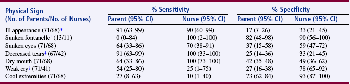
*The total number of patients for this outcome equals 71. Three patients from the subset of 71 did not have nursing assessments for physical signs completed.
†Subset of 32 infants <9 months of age with only 2 cases of significant dehydration.
‡Parents and nurses could answer “no opportunity to observe,” resulting in missing data for parents (4 patients) and nurses (26 patients).
§Nurses could answer “no opportunity to observe,” resulting in missing data (27 patients).
From Porter, S. C., Fleisher, G.R., Kohane, I. S., & Mandl, K. D. (2003). The value of parental report for diagnosis and management of dehydration in the emergency department. Annals of Emergency Medicine, 41(2), 202.
Likelihood ratios (LRs) are additional calculations that can help researchers to determine the accuracy of diagnostic or screening tests, which are based on the sensitivity and specificity results. The LRs are calculated to determine the likelihood that a positive test result is a true positive and a negative test result is a true negative. The ratio of the true positive results to false positive results is known as the positive LR (Craig & Smyth, 2007). The positive LR is calculated as follows:

The negative LR is the ratio of true negative results to false negative results, and it is calculated as follows:

The very high LRs (or those that are above 10) rule in the disease or indicate that the patient has the disease. The very low LRs (or those that are < 0.1) virtually rule out the chance that the patient has the disease (Melnyk & Fineout-Overholt, 2005). Understanding sensitivity, specificity, and LR increases your ability to read clinical studies and to determine the most accurate diagnostic test to use in clinical practice.
VALIDITY IN QUALITATIVE RESEARCH
One of the most serious concerns related to qualitative research has been the lack of strategies to determine the validity of the measurements that led to the development of theory. Qualitative researchers tend to work alone. Biases in their work, which threaten validity, can easily go undetected. Miles and Huberman (1994) have cautioned the qualitative researcher to be alert to the occurrence of the holistic fallacy. This fallacy occurs as the researcher becomes more and more sure that his or her conclusions are correct and that the model does, in fact, explain the situation. This feeling should arouse suspicion and alert the researcher to validate his or her findings. Miles and Huberman (1994) have described 12 strategies for examining the validity of qualitative measures:
Checking for representativeness. Qualitative measurement can be biased by either the attention of the researcher or a bias in the people from whom they obtain their measures. To ensure that measures are representative of the entire population, the researcher looks for sources of data not easily accessible. The researcher assumes that observed actions are representative of actions that occur when the researcher is not present. However, efforts must be made to determine whether this is so.
Checking for researcher effects. In many cases, the researcher’s presence can alter behavior, leading to invalid measures. To avoid this effect, the researcher must (1) remain on the site long enough to become familiar, (2) use unobtrusive measures, and (3) seek input from informants or study participants.
Triangulating. The qualitative researcher must compare all the measures from different sources to determine the validity of the findings.
Weighing the evidence. Qualitative research involves reducing large amounts of data during the process of coming to conclusions. In this process, some evidence is captured from this mass of data and is used in reaching conclusions. The researcher needs to review the strength of the captured data to validate the conclusions. The researcher determines the strength of the evidence from the source, the circumstances of data collection, and the researcher’s efforts to validate the evidence. The researcher must search actively for reasons why the evidence should not be trusted.
Making contrasts and comparisons. Contrasts between subjects or events in relation to the study conclusions must be examined. An example would be an action that nursing supervisors consider to be very important but that staff nurses regard as simply another administrative activity. The two extreme positions must be examined. A decision must then be made about whether the difference is a significant one.
Checking the meaning of outliers. Exceptions to findings must be identified and examined. These exceptions are referred to as outliers. The outliers provide a way to test the generality of the findings. Therefore, in the selection of subjects, it may be important to seek individuals who seem to be outliers.
Using extreme cases. Certain types of outliers, referred to as extreme cases, can be useful in confirming conclusions. The researcher can compare the extreme case with the theoretical model that was developed and determine the key factor that causes the model not to fit the case. Purposive sampling is often used to ensure that extreme cases are included.
Ruling out spurious relations. The strategy of ruling out spurious relations requires the examination of relationships identified in the model to consider the possibility of a third variable influencing the situation.
Replicating a finding. Documenting the findings from several independent sources increases the dependability of the findings and diminishes the risk of the holistic fallacy. The findings can be tested either with new data collected later in the study or with data from another site or data set. The second option is more rigorous.
Checking out rival explanations. The qualitative researcher is taught to keep several hypotheses in mind and constantly to compare the plausibility of each with the possibility that one of the others is more accurate. Near the end of data analysis, however, when the researcher is more emotionally “wedded to” one idea, it is useful to have someone not involved in the research act as a devil’s advocate. Questions such as “What could disprove the hypothesis?” or, conversely, “What does the present hypothesis disprove?” should be asked. Evidence that does not fit the hypothesis must be carefully examined.
Looking for negative evidence. A search for negative evidence naturally flows from the searches for outliers and rival explanations. In this step, there is an active search for disconfirmation of what is believed to be true. The researcher goes back through the data, seeking evidence to disconfirm the conclusions. However, the inability to find disconfirming evidence never decisively confirms the conclusions reached by the researcher. In some cases, independent verification, through examination of the data by a second qualitative researcher, is sought.
Obtaining feedback from informants or study participants. Conclusions should be given to the participants, and feedback is sought from them about the accuracy of the causal network developed. Although researchers have been getting feedback from participants throughout the analysis period, feedback after completion of the model provides a different type of verification of the information.
SUMMARY
• Measurement is the process of assigning numbers to objects, events, or situations in accord with some rule.
• Instrumentation is the application of specific rules to develop a measurement device or instrument.
• Measurement theory and the rules within this theory have been developed to direct the measurement of abstract and concrete concepts.
• There is direct measurement and indirect measurement.
• Health care technology has made researchers familiar with direct measures of concrete elements, such as height, weight, heart rate, temperature, and blood pressure, very familiar.
• Indirect measurement is used with abstract concepts, when the concepts are not measured directly, but when the indicators or attributes of the concepts are used to represent the abstraction.
• Measurement error is the difference between what exists in reality and what is measured by a research instrument.
• The levels of measurement, from lower to higher, are nominal, ordinal, interval, and ratio.
• Reliability refers to how consistently the measurement technique measures the concept of interest.
• The validity of an instrument is determined by the extent to which the instrument actually reflects the abstract construct being examined.
• Evaluation of physiological measures requires a different perspective from that of behavioral measures and requires evaluation for accuracy, precision, selectivity, and sensitivity.
• The accuracy of screening or diagnostic tests is determined by calculating the sensitivity, specificity, and likelihood ratios for the test.
• One of the most serious concerns related to qualitative research has been the lack of strategies to determine the validity of the measurements that led to the development of theory. However, strategies are being identified to examine the validity of qualitative measures.
American Psychological Association’s Committee to Develop Standards. Standards for educational and psychological testing. Washington, DC: American Psychological Association, 1985.
Armstrong, G.D. Parametric statistics and ordinal data: A pervasive misconception. Nursing Research. 1981;30(1):60–62.
Armstrong, G.D. Parametric statistics [Letter]. Nursing Research. 1984;33(1):54.
Bakas, T., Champion, V., Perkins, S.M., Farran, C.J., Williams, L.S. Psychometric testing of the revised 15-item Bakas Caregiving Outcomes Scale. Nursing Research. 2006;55(5):346–355.
Berk, R.A. Importance of expert judgment in content-related validity evidence. Western Journal of Nursing Research. 1990;12(5):659–671.
Brinberg, D., McGrath, J.E. Validity and the research process. Beverly Hills, CA: Sage, 1985.
Campbell, D.T., Fiske, D.W. Convergent and discriminant validation by the multitrait-multimethod matrix. Psychological Bulletin. 1959;56(2):81–105.
Cohen, J.A. A coefficient of agreement for nominal scales. Education and Psychological Measurement. 1960;20(1):37–46.
Craig, J.V., Smyth, R.L. The evidence-base practice manual for nurses, (2nd ed.). Edinburgh, Scotland: Churchill Livingstone; 2007.
Davis, L.L. Instrument review: Getting the most from a panel of experts. Applied Nursing Research. 1992;5(4):194–197.
DeKeyser, F.G., Pugh, L.C. Assessment of the reliability and validity of biochemical measures. Nursing Research. 1990;39(5):314–317.
DeVellis, R.F. Scale development: Theory and applications. Newbury Park, CA: Sage, 1991.
Engstrom, J.L. Assessment of the reliability of physical measures. Research in Nursing & Health. 1988;11(6):383–389.
Estok, P.J., Sedlak, C.A., Doheny, M.O., Hall, R. Structural model for osteoporosis preventing behavior in postmenopausal women. Nursing Research. 2007;56(3):149–158.
Garvin, B.J., Kennedy, C.W., Cissna, K.N. Reliability in category coding systems. Nursing Research. 1988;37(1):52–55.
Gift, A.G., Soeken, K.L. Assessment of physiologic instruments. Heart & Lung. 1988;17(2):128–133.
Goodwin, L.D., Goodwin, W.L. Estimating construct validity. Research in Nursing & Health. 1991;14(3):235–243.
Grove, S.K. Statistics for health care research: A practical workbook. Philadelphia: Saunders, 2007.
Guetzkow, H. Unitizing and categorizing problems in coding qualitative data. Journal of Clinical Psychology. 1950;6(1):47–58.
Gunning, R., Kallan, R.A. How to take the fog out of business writing. Chicago: Dartnell, 1994.
Hagerty, B.M.K., Patusky, K. Developing a measure of sense of belonging. Nursing Research. 1995;44(1):9–13.
Imle, M.A., Atwood, J.R. Retaining qualitative validity while gaining reliability and validity: Development of the Transition to Parenthood Concerns Scale. Advanced Nursing Science. 1988;11(1):61–75.
Johnson, M.J. The development and testing of three medication-taking questionnaires for the medication adherence model constructs for hypertensive patients.Unpublished doctoral dissertation. University of Utah, Salt Lake City: UT, 2002.
Johnson, M.J., Rogers, S. Development of the Purposeful Action Medication-Taking Questionnaire. Western Journal of Nursing Research. 2006;28(3):335–351.
Johnson, M.J., Williams, M., Marshall, E.S. Adherent and nonadherent medication-taking elderly hypertensive patients. Clinical Nursing Research. 1999;8(4):318–335.
Kaplan, A. The conduct of inquiry: Methodology for behavioral science. New York: Harper & Row, 1963.
Knapp, T.R. Parametric statistics [Letter]. Nursing Research. 1984;33(1):54.
Knapp, T.R. Treating ordinal scales as interval scales: An attempt to resolve the controversy. Nursing Research. 1990;39(2):121–123.
Lynn, M.R. Determination and quantification of content validity. Nursing Research. 1986;35(6):382–385.
Marshall, C., Rossman, G.B. Designing qualitative research, (4th ed.). Thousand Oaks, CA: Sage; 2006.
Melnyk, B.M., Fineout-Overholt, E. Evidence-based practice in nursing & healthcare: A guide to best practice. Philadelphia: Lippincott Williams & Wilkins, 2005.
Miles, M.B., Huberman, A.M. Qualitative data analysis: A sourcebook of new methods, (2nd ed.). Beverly Hills, CA: Sage; 1994.
Miller, B., Bodie, M. Determination of reading comprehension level for effective patient health-education materials. Nursing Research. 1994;43(2):118–119.
Miller, T.W. Life events scaling: Clinical methodological issues. Nursing Research. 1981;30(5):316–320A.
Munro, B.H. Statistical methods for health care research, (3rd ed.). Philadelphia: Lippincott; 2001.
Nagley, S.J., Byers, P.H. Clinical construct validity. Journal of Advanced Nursing. 1987;12(5):617–619.
National Osteoporosis Foundation (NOF). Stand up to osteoporosis [Brochure]. Washington, DC: Author, 2003.
Nunnally, J.C., Bernstein, I.H. Psychometric theory, (3rd ed.). New York: McGraw-Hill; 1994.
Porter, S.C., Fleisher, G.R., Kohane, I.S., Mandl, K.D. The value of parental report for diagnosis and management of dehydration in the emergency department. Annals of Emergency Medicine. 2003;41(2):196–205.
Rasin, J.H. Measurement issues with the elderly. In: Frank-Stromberg M., Olsen S.J, eds. Instruments for clinical health-care research. (2nd ed.). Boston: Jones & Bartlett; 1997:44–53.
Rew, L., Stuppy, D., Becker, H. Construct validity in instrument development: A vital link between nursing practice, research, and theory. Advances in Nursing Science. 1988;10(4):10–22.
Silvaroli, N.J. Classroom reading inventory, (5th ed.). Dubuque, IA: William C.Brown; 1986.
Stevens, S.S. On the theory of scales of measurement. Science. 1946;103(2684):677–680.
Stommel, M., Wang, S., Given, C.W., Given, B. Confirmatory factor analysis (CFA) as a method to assess measurement equivalence. Research in Nursing & Health. 1992;15(5):399–405.
Streiner, D.L., Norman, G.R. Health measurement scales: A practical guide to their development and use, (2nd ed.). Oxford, England: Oxford University Press; 1995.
Teel, C., Verran, J.A. Factor comparison across studies. Research in Nursing & Health. 1991;14(1):67–72.
Thomas, S.D., Hathaway, D.K., Arheart, K.L. Face validity. Western Journal of Nursing Research. 1992;14(1):109–112.
Topf, M. Interrater reliability decline under covert assessment. Nursing Research. 1988;37(1):47–49.
Wahner, H.W., Fogelman, I. The evaluation of osteoporosis: Dual energy x-ray absorptiometry in clinical practice. In: Wahner H.W., Fogleman I., eds. Mayo clinic proceedings. London: Mayo Clinic; 1994:178–195.
Waltz, C.W., Bausell, R.B. Nursing Research: Design, statistics and computer analysis. Philadelphia: F.A.Davis, 1981.
Washington, C.C., Moss, M. Pragmatic aspects of establishing interrater reliability in research. Nursing Research. 1988;37(3):190–191.
World Health Organization Study Group. Assessment of fracture risk and its application to screening for postmenopausal osteoporosis. Geneva, Switzerland: World Health Organization, 1994.