Introduction to Statistical Analysis
Data analysis is probably the most exciting part of research. During this phase, you will finally obtain answers to the questions that initially generated your research activity. Nevertheless, nurses probably experience greater anxiety about this phase of the research process than any other, as they question issues that range from their knowledge about critiquing published studies to their ability to conduct research. To critique a quantitative study, you need to be able to (1) identify the statistical procedures used; (2) judge whether these statistical procedures were appropriate for the hypotheses, questions, or objectives of the study and for the data available for analysis; (3) comprehend the discussion of data analysis results; (4) judge whether the author’s interpretation of the results is appropriate; and (5) evaluate the clinical significance of the findings. A neophyte researcher performing a quantitative study is confronted with many critical decisions related to data analysis that require statistical knowledge. To perform statistical analysis of data from a quantitative study, you need to be able to (1) prepare the data for analysis; (2) describe the sample; (3) test the reliability of measures used in the study; (4) perform exploratory analyses of the data; (5) perform analyses guided by the study objectives, questions, or hypotheses; and (6) interpret the results of statistical procedures. Critiquing studies and performing statistical analyses both require an understanding of the statistical theory underlying the process of analysis.
This chapter and the following five will provide you with the information needed to critique the statistical sections of published studies or perform statistical procedures. This chapter introduces the concepts of statistical theory and discusses some of the more pragmatic aspects of quantitative data analysis: the purposes of statistical analysis, the process of performing data analysis, the method for choosing appropriate statistical procedures for a study, and resources for statistical analysis. Chapter 19 explains the use of statistics for descriptive purposes; Chapter 20 discusses the use of statistics to test proposed relationships; Chapter 21 explores the use of statistics for prediction; and Chapter 22 guides you in using statistics to examine causality.
CONCEPTS OF STATISTICAL THEORY
One reason that nurses tend to avoid statistics is that many were taught only the mathematical mechanics of calculating statistical formulas and were given little or no explanation of the logic behind the analysis procedure or the meaning of the results. This mechanical process is usually performed by computer, and information about it offers little assistance to those making statistical decisions or explaining results. We will approach data analysis from the perspective of enhancing your understanding of the meaning underlying statistical analysis. You can then use this understanding either to critique or to perform data analyses.
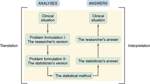
As is common in many theories, theoretical ideas related to statistics are expressed by unique terminology and logic that is unfamiliar to many. Research ideas (particularly data analysis as expressed in the language of the clinician and the researcher) are perceived by statisticians to be relatively imprecise and vague because they are not expressed in the formal language of the professional statistician. To resolve this language barrier, it is necessary to translate a data analysis plan from the common language (or even general research language) to the language of statisticians. When the analysis is complete, the results must be translated from the language of the statistician back to the language of the researcher and the clinician. Thus, explaining the results is a process of interpretation (Chervany, 1977). Figure 18-1 illustrates this process of translation and interpretation.
The ensuing discussion explains some of the concepts commonly used in statistical theory. The logic of statistical theory is embedded within the explanations of these concepts. The concepts presented include probability theory, decision theory, inference, the theoretical normal curve, sampling distributions, sampling distribution of a statistic, shapes of distributions, standardized scores, confidence intervals, statistics and parameters, samples and populations, estimation of parameters, degrees of freedom, tailedness, type I and type II errors, level of significance, power, clinical significance, parametric and nonparametric statistical analyses, causality, and relationships.
Probability Theory
Probability theory addresses statistical analysis as the likelihood of accurately predicting an event or the extent of a relationship. Nurse researchers might be interested in the probability of a particular nursing outcome in a particular patient care situation. With probability theory, you could determine how much of the variation in your data could be explained by using a particular statistical analysis. In probability theory, the researcher interprets the meaning of statistical results in light of his or her knowledge of the field of study. A finding that would have little meaning in one field of study might be important in another (Good, 1983). Probability is expressed as a lowercase p, with values expressed as percentages or as a decimal value ranging from 0 to 1. If the exact probability is known to be 0.23, for example, it would be expressed as p = 0.23.
Decision Theory and Hypothesis Testing
Decision theory is inductive in nature and is based on assumptions associated with the theoretical normal curve. When using decision theory, one always begins with the assumption that all the groups are members of the same population. This assumption is expressed as a null hypothesis. See Chapter 8 for an explanation of null hypothesis. To test the assumption, a cutoff point is selected before data collection. This cutoff point, referred to as alpha (α), or the level of significance, is the point on the normal curve at which the results of statistical analysis indicate a statistically significant difference between the groups. Decision theory requires that the cutoff point be absolute. Thus, the meaning applied to the statistical results is not based on the researcher’s interpretation. Absolute means that even if the value obtained is only a fraction above the cutoff point, the samples are considered to be from the same population and no meaning can be attributed to the differences. Thus, it is inappropriate when using this theory to make a statement that “the findings approached significance at the 0.051 level” if the alpha level was set at 0.05. By decision theory rules, this finding indicates that the groups tested are not significantly different and the null hypothesis is accepted. On the other hand, if the analysis reveals a significant difference of 0.001, this result is not more significant than the 0.05 originally proposed (Slakter, Wu, & Suzuki-Slakter, 1991).
Inference
Statisticians use the term inference or infer in somewhat the same way that a researcher uses the term generalize. Inference requires the use of inductive reasoning. One infers from a specific case to a general truth, from a part to the whole, from the concrete to the abstract, from the known to the unknown. When using inferential reasoning, you can never prove things; you can never be certain. However, one of the reasons for the rules that have been established with regard to statistical procedures is to increase the probability that inferences are accurate. Inferences are made cautiously and with great care.
Normal Curve
The theoretical normal curve is an expression of statistical theory. It is a theoretical frequency distribution of all possible scores. However, no real distribution exactly fits the normal curve. The idea of the normal curve was developed by an 18-year-old mathematician, Johann Gauss, in 1795, who found that data measured repeatedly in many samples from the same population by using scales based on an underlying continuum can be combined into one large sample. From this large sample, one can develop a more accurate representation of the pattern of the curve in that population than is possible with only one sample. Surprisingly, in most cases, the curve is similar, regardless of the specific data that have been examined or the population being studied.
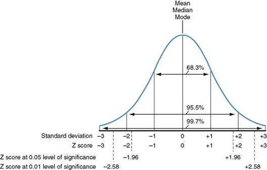
This theoretical normal curve is symmetrical and unimodal and has continuous values. The mean, median, and mode (summary statistics) are equal (Figure 18-2). The distribution is completely defined by the mean and standard deviation. The measures in the theoretical distribution have been standardized by using Z scores. These terms are explained further in Chapter 19. Note the Z scores and standard deviation (SD) values indicated in Figure 18-2. The proportion of scores that may be found in a particular area of the normal curve has been identified. In a normal curve, 68% of the scores will be within 1 SD or 1 Z score above or below the mean, 95% will be within 1.96 SD above or below the mean, and more than 99% will be within 2.58 SD above or below the mean. Even when statistics, such as means, come from a population with a skewed (asymmetrical) distribution, the sampling distribution developed from multiple means obtained from that skewed population will tend to fit the pattern of the normal curve. This phenomenon is referred to as the central limit theorem. One requirement for the use of parametric statistical analysis is that the data must be normally distributed—normal meaning that the data approximately fit the normal curve. Many statistical measures from skewed samples also fit the normal curve because of the central limit theorem; thus, some statisticians believe that it is justifiable to use parametric statistical analysis even with data from skewed samples if the sample is large enough (Volicer, 1984).
Sampling Distributions
A distribution is the state or manner in which values are arranged within the data set. A sampling distribution is the manner in which statistical values (such as means), obtained from multiple samples of the same population, are distributed within the set of values. The mean of this type of distribution is referred to as the mean of means (). Sampling distributions can also be developed from standard deviations. Other values, such as correlations between variables, scores obtained from specific measures, and scores reflecting differences between groups within the population, can yield values that can be used to develop sampling distributions.
The sampling distribution allows us to estimate sampling error. Sampling error is the difference between the sample statistic used to estimate a parameter and the actual, but unknown, value of the parameter. If we know the sampling distribution of a statistic, it allows us to measure the probability of making an incorrect inference. One should never make an inference without being able to calculate the probability of making an incorrect inference.
Sampling Distribution of a Statistic
Just as it is possible to develop distributions of summary statistics within a population, it is possible to develop distributions of inferential statistical outcomes. For example, if you repeatedly obtained two samples of the same size from the same population and tested for differences in the means with a t-test, you could develop a sampling distribution from the resulting t values by using probability theory. With this approach, you could develop a distribution for samples of many varying sizes. Such a distribution has, in fact, been generated by using t values. A table of t distribution values is available in Appendix C. Tables have been developed with this strategy to organize the statistical outcomes of many statistical procedures from various sample sizes. Because listing all possible outcomes would require many pages, most tables include only values that have a low probability of occurring in the present theoretical population. These probabilities are expressed as alpha (α), commonly referred to as the level of significance, and as beta (β), the probability of a type II error.
By using the appropriate sampling distribution, you could determine the probability of obtaining a specific statistical result if the two samples you have been studying are really from the same population. Statistical analysis makes an inference that the samples being tested can be considered part of the population from which the sampling distribution was developed. This inference is expressed as a null hypothesis.
The Shapes of Distributions
The shape of the distribution provides important information about the data. The outline of the distribution shape is obtained by using a histogram. Within this outline, the mean, median, mode, and standard deviation can then be graphically illustrated (see Figure 18-2). This visual presentation of combined summary statistics provides insight into the nature of the distribution. As the sample size becomes larger, the shape of the distribution will more accurately reflect the shape of the population from which the sample was taken.
Symmetry
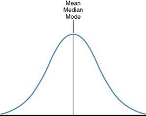
Several terms are used to describe the shape of the curve (and thus the nature of a particular distribution). The shape of a curve is usually discussed in terms of symmetry, skewness, modality, and kurtosis. A symmetrical curve is one in which the left side is a mirror image of the right side (Figure 18-3). In these curves, the mean, median, and mode are equal and are the dividing point between the left and right sides of the curve.
Skewness
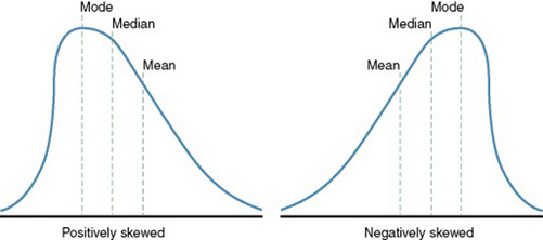
Any curve that is not symmetrical is referred to as skewed or asymmetrical. Skewness may be exhibited in the curve in a variety of ways (Figure 18-4). A curve may be positively skewed, which means that the largest portion of data is below the mean. For example, data on length of enrollment in hospice are positively skewed. Most of the people die within the first 3 weeks of enrollment, whereas increasingly smaller numbers survive as time increases. A curve can also be negatively skewed, which means that the largest portion of data is above the mean. For example, data on the occurrence of chronic illness by age in a population are negatively skewed, with most chronic illnesses occurring in older age groups.
In a skewed distribution, the mean, median, and mode are not equal. Skewness interferes with the validity of many statistical analyses; therefore, statistical procedures have been developed to measure the skewness of the distribution of the sample being studied. Few samples will be perfectly symmetrical; however, as the deviation from symmetry increases, the seriousness of the impact on statistical analysis increases. A popular skewness measure is expressed in the following equation:
In this equation, a result of zero indicates a completely symmetrical distribution, a positive number indicates a positively skewed distribution, and a negative number indicates a negatively skewed distribution. Statistical analyses conducted by computer often automatically measure skewness, which is then indicated on the computer printout. Strongly skewed distributions often must be analyzed by nonparametric techniques, which make no assumptions of normally distributed samples. In a positively skewed distribution, the mean is greater than the median, which is greater than the mode. In a negatively skewed distribution, the mean is less than the median, which is less than the mode. There is no firm rule about when data are sufficiently skewed to require the use of nonparametric techniques. The researcher and the statistician should make this decision jointly.
Modality
Another characteristic of distributions is their modality. Most curves found in practice are unimodal, which means that they have one mode and frequencies progressively decline as they move away from the mode. Symmetrical distributions are usually unimodal. However, curves can also be bimodal (Figure 18-5) or multimodal. When you find a bimodal sample, it usually means that you have not adequately defined your population.

Kurtosis
Another term used to describe the shape of the distribution curve is kurtosis. Kurtosis explains the degree of peakedness of the curve, which is related to the spread of variance of scores. An extremely peaked curve is referred to as leptokurtic, an intermediate degree of kurtosis as mesokurtic, and a relatively flat curve as platykurtic (Figure 18-6). Extreme kurtosis can affect the validity of statistical analysis because the scores have little variation. Many computer programs analyze kurtosis before conducting statistical analysis. A common equation used to measure kurtosis is
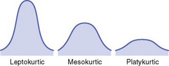
A kurtosis of zero indicates that the curve is mesokurtic. Values below zero indicate a platykurtic curve (Box, Hunter, & Hunter, 1978). There is no firm rule about when data are sufficiently kurtotic to affect the validity of the statistical procedures. The researcher and the statistician should make this decision jointly.
Standardized Scores
Because of differences in the characteristics of various distributions, comparing a score in one distribution with a score in another distribution is difficult. For example, if you were comparing test scores from two classroom examinations and one test had a high score of 100 and the other had a high score of 70, the scores would be difficult to compare. To facilitate this comparison, a mechanism has been developed to transform raw scores into standard scores. Numbers that make sense only within the framework of the measurements used within a specific study are transformed into numbers (standard scores) that have a more general meaning. Transformation to standard scores makes it easier for those evaluating the numbers to conceptually grasp of the meaning of the score.
A common standardized score is called a Z score. It expresses deviations from the mean (difference scores) in terms of standard deviation units. The equation for a Z score is
A score that falls above the mean will have a positive Z score, whereas a score that falls below the mean will have a negative Z score (see Figure 18-2). The mean expressed as a Z score is zero. The SD of Z scores is 1. Thus, a Z score of 2 indicates that the score from which it was obtained is 2 SD above the mean. A Z score of -0.5 indicates that the score was 0.5 SD below the mean. The larger the absolute value of the Z score, the less likely the observation is to occur. For example, a Z score of 4 would be extremely unlikely. The cumulative normal distribution expressed in Z scores is provided in Appendix B.
Confidence Intervals
When the probability of including the value of the parameter within the interval estimate is known (as described in Chapter 19), it is referred to as a confidence interval. Calculating the confidence interval involves the use of two formulas to identify the upper and lower ends of the interval. The formula for a 95% confidence interval when sampling from a population with a known standard deviation or from a normal population with a sample size greater than 30 is
If you had a sample with a mean of 40, an SD of 5, and an N of 50, you would be able to calculate a confidence interval:
Confidence intervals are usually expressed as “(38.6, 41.4),” with 38.6 being the lower end and 41.4 being the upper end of the interval. Theoretically, we can produce a confidence interval for any parameter of a distribution. It is a generic statistical procedure. For example, confidence intervals can also be developed around correlation coefficients (Glass & Stanley, 1970). Estimation can be used for a single population or for multiple populations. In estimation, we are inferring the value of a parameter from sample data and have no preconceived notion of the value of the parameter. In contrast, in hypothesis testing we have an a priori theory about the value of the parameter or parameters or some combination of parameters.
Statistics and Parameters, Samples and Populations
Use of the terms statistic and parameter can be confusing because of the various populations referred to in statistical theory. A statistic (–x) is a numerical value obtained from a sample. A parameter is a true (but unknown) numerical characteristic of a population. For example, is the population mean or arithmetic average. The mean of the sampling distribution (mean of samples’ means) can also be shown to be equal to. Thus, a numerical value that is the mean (–x) of the sample is a statistic; a numerical value that is the mean of the population is a parameter (Barnett, 1982).
Relating a statistic to a parameter requires an inference as one moves from the sample to the sampling distribution and then from the sampling distribution to the population. The population referred to is in one sense real (concrete) and in another sense abstract. These ideas are illustrated as follows:

For example, perhaps you are interested in the cholesterol level of women in the United States. Your population is women in the United States. Obviously, you cannot measure the cholesterol level of every woman in the United States; therefore, you select a sample of women from this population. Because you wish your sample to be as representative of the population as possible, you obtain your sample by using random sampling techniques. To determine whether the cholesterol levels in your sample are like those in the population, you must compare the sample with the population. One strategy would be to compare the mean of your sample with the mean of the entire population. Unfortunately, it is highly unlikely that you know the mean of the entire population. Therefore, you must make an estimate of the mean of that population. You need to know how good your sample statistics are as estimators of the parameters of the population.
First, you make some assumptions. You assume that the mean scores of cholesterol levels from multiple randomly selected samples of this population would be normally distributed. This assumption implies another assumption: that the cholesterol levels of the population will be distributed according to the theoretical normal curve—that difference scores and standard deviations can be equated to those in the normal curve.
If you assume that the population in your study is normally distributed, you can also assume that this population can be represented by a normal sampling distribution. Thus, you infer from your sample to the sampling distribution, the mathematically developed theoretical population made up of parameters such as the mean of means and the standard error. The parameters of this theoretical population are those measures of the dimensions identified in the sampling distribution. You can then infer from the sampling distribution to the population. You have both a concrete population and an abstract population. The concrete population consists of all those individuals who meet your sampling criteria, whereas the abstract population consists of individuals who will meet your sampling criteria in the future or those groups addressed theoretically by your framework.
Estimation of Parameters
You may use two approaches to estimate the parameters of a population: point estimation and interval estimation.
Point Estimation
A statistic that produces a value as a function of the scores in a sample is called an estimator. Much of inferential statistical analysis involves the use of point estimation to evaluate the fit between the estimator (a statistic) and the population parameter. A point estimate is a single figure that estimates a related figure in the population of interest. The best point estimator of the population mean is the mean of the sample being examined. However, the mean of the sample rarely equals the mean of the population. In addition to the mean, other commonly used estimators include the median, variance, standard deviation, and correlation coefficient.
Interval Estimation
When sampling from a continuous distribution, the probability of the sample mean being exactly equal to the population mean is zero. Therefore, we know that we are going to be in error if we use point estimators. The difference between the sample estimate and the true, but unknown, parameter value is sampling error. The source of sampling error is the fact that we did not count every individual in the population. Sampling error is due to chance and chance alone. It is not due to some flaw in the researcher’s methodology. Interval estimation is an attempt to overcome this problem by controlling the initial precision of an estimator. An interval procedure that gives a 95% level of confidence will produce a set of intervals, 95% of which will include the true value of the parameter. Unfortunately, after a sample is drawn and the estimate is calculated, it is not possible to tell whether the interval contains the true value of the parameter.
An interval estimate is a segment of a number line (or range of scores) where the value of the parameter is thought to be. For example, in a sample with a mean of 40 and an SD of 5, one might use the range of scores between 2 SD below the mean to 2 SD above the mean (30 to 50) as the interval estimation. This type of estimation provides a set of scores rather than a single score. However, it is not absolutely certain that the mean of the population lies within that range. Therefore, it is necessary to determine the probability that this interval estimate contains the population mean.
This need to determine probability brings us back to the sampling distribution. We know that 95% of the means in the sampling distribution lie within ±1.96 SD of the mean of means (the population mean). If these scores are converted to Z scores, the unit normal distribution table can be used to determine how many standard deviations out from the mean of means one must go to ensure a specified probability (e.g., 70%, 95%, or 99%) of obtaining an interval estimate that includes the population parameter that is being estimated.
By examining the normal distribution (see Figure 18-2), one finds that 2.5% of the area under the normal curve lies below a Z score of -1.96, or μ -  , and 2.5% of the area lies above a Z score of 1.96, or μ + (1.96
  ), where μ is the mean of means, SD is the standard deviation, and N is the sample size. The probability is 0.95 that a randomly selected sample would have a mean within this range. Calculation of confidence intervals is explained in Chapter 19.
Degrees of Freedom
The concept of degrees of freedom (df) is a product of statistical theory and is easier to calculate than it is to explain because of the complex mathematics involved to justify the concept. Degrees of freedom involve the freedom of a score’s value to vary given the other existing scores’ values and the established sum of these scores.
A simple example may begin to explain the concept. Suppose difference scores are obtained from a sample of 4 and the mean is 4. The difference scores are -2, -1, +1, and +2. As with all difference scores, the sum of these scores is 0. As a result, if any three of the difference scores are calculated, the value of the fourth score is not free to vary. Its value will depend on the values of the other three to maintain a mean of 4 and a sum of 0. The degree of freedom in this example is 3 because only three scores are free to vary. In this case and in many other analyses, the degree of freedom is the sample size (N) minus 1 (N - 1).
In this example, df = 4 - 1 = 3 (Roscoe, 1969). In some analyses, determining levels of significance from tables of statistical sampling distributions requires knowledge of the degrees of freedom.
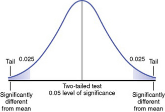
Tailedness
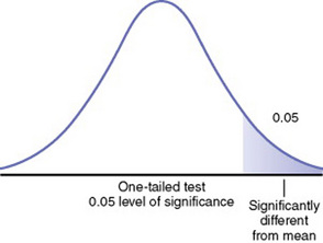
On a normal curve, extremes of statistical values can occur at either end of the curve. Therefore, the 5% of statistical values that are considered statistically significant according to decision theory must be distributed between the two extremes of the curve. The extremes of the curve are referred to as tails. If the hypothesis is nondirectional and assumes that an extreme score can occur in either tail, the analysis is referred to as a two-tailed test of significance (Figure 18-7).
In a one-tailed test of significance, the hypothesis is directional, and extreme statistical values that occur in a single tail of the curve are of interest. Developing a one-tailed hypothesis requires sufficient knowledge of the variables and their interaction on which to base a one-tailed test. Otherwise, the one-tailed test is inappropriate. This knowledge may be theoretical or from previous research. (Refer to Chapter 8 for formulating hypotheses.) One-tailed tests are uniformly more powerful than two-tailed tests, and this fact increases the possibility of rejecting the null hypothesis. In this case, extreme statistical values occurring on the other tail of the curve are not considered significantly different. In Figure 18-8, which is a one-tailed figure, the portion of the curve where statistical values will be considered significant is in the right tail of the curve.
Type I and Type II Errors
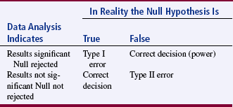
According to decision theory, two types of error can occur when making decisions about the meaning of a value obtained from a statistical test: type I errors and type II errors. A type I error occurs if the null hypothesis is rejected when, in fact, it is true. This error is possible because even though statistical values in the extreme ends of the tail of the curve are rare, they do occur within the population. In viewing Table 18-1, remember that the null hypothesis states that there is no difference or no association between groups.
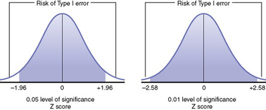
The risk of making a type I error is greater with a 0.05 level of significance than with a 0.01 level. As the level of significance becomes more extreme, the risk of a type I error decreases, as illustrated in Figure 18-9. For example, suppose you studied the effect of a treatment in an experimental study consisting of two groups and found that the difference between the two groups was relatively equivalent in magnitude to the standard error. The sampling distribution of the difference between the group means tells you that even if there is no real difference between the groups, a difference as large as or larger than the one you detected would occur by chance about once in every three times. That is, the difference that you found is just what you could expect to occur if the true treatment effect were zero. This statement does not mean that the true difference is zero, but that on the basis of the results of the study you would not be justified in claiming a real difference between the groups. The data from your samples do not establish a case for the position that a true treatment effect exists.
Suppose, on the other hand, that you find that the difference in your groups is over twice its standard error (Z score >1.96). (Examine the Z scores in Figure 18-2.) A treatment difference of this magnitude would occur by chance less than 1 time in 20, and we say that these results are statistically significant at the 0.05 level. A difference of more than 2.58 times the standard error would occur by chance less than 1 time in 100, and we say that the difference is statistically significant at the 0.01 level. Cox (1958) stated, “Significance tests, from this point of view, measure the adequacy of the data to support the qualitative conclusion that there is a true effect in the direction of the apparent difference” (p.159). Thus, the decision is a judgment and can be in error. The level of statistical significance attained indicates the degree of uncertainty in taking the position that the difference between the two groups is real.
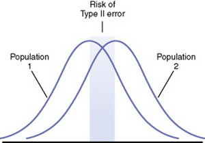
A type II error occurs if the null hypothesis is regarded as true when, in fact, it is false. This type of error occurs as a result of some degree of overlap between the values of different populations in some cases, so a value with a greater than 5% probability of being within one population may in fact be within the dimensions of another population (Figure 18-10).
As the risk of a type I error decreases (by setting a more extreme level of significance), the risk of a type II error increases. When the risk of a type II error decreases (by setting a less extreme level of significance), the risk of a type I error increases. It is not possible to decrease both types of error simultaneously without a corresponding increase in sample size. Therefore, the researcher needs to decide which risk poses the greatest threat within a specific study. In nursing research, many studies are conducted with small samples and instruments that are not precise measures of the variables under study. Many nursing situations include multiple variables that interact to lead to differences within populations. However, when one is examining only a few of the interacting variables, small differences can be overlooked and could lead to a false conclusion of no differences between the samples. In this case, the risk of a type II error is a greater concern, and a more lenient level of significance is in order.
As an example of the concerns related to error, consider the following problem. If you were to obtain three samples by using the same methodology, each sample would have a different mean. Yet you need to make a decision to accept or reject the null hypothesis. The null hypothesis states that the population mean is 50 and that the three samples shown here are all from the same population. Assume that you obtain the following results:


How much evidence would it take to convince you to switch from believing the null hypothesis to believing the alternative hypothesis? Will you choose correctly, or will you make a type I or a type II error?
Level of Significance: Controlling the Risk of a Type I Error
The formal definition of the level of significance (α) is the probability of making a type I error when the null hypothesis is true. The level of significance, developed from decision theory, is the cutoff point used to determine whether the samples being tested are members of the same population or from different populations. The decision criteria are based on the selected level of significance and the sampling distribution of the mean. For this example, we assume that the sampling distribution of the mean is normally distributed. As mentioned previously, 68% of the means from samples in a population will fall within 1SD of the mean of means (μ), 95% will fall within 1.96SD, 99% within 2.58SD, and 99.7% within 3SD. This decision theory explanation of the expected distribution of means is equivalent to the confidence interval explanation described previously. It is simply expressed differently. In keeping with decision theory, the level of significance sought in a statistical test must be established before conducting the test. In fact, the significance level needs to be established before collecting the data. In nursing studies, the level of significance is usually set at 0.05 or 0.01. However, in preliminary studies, it might be prudent to select a less stringent level of significance, such as 0.10.
If one wishes to predict with a 95% probability of accuracy, the level of significance would be p ≤1–0.95, or p ≤ 0.05. The mathematical symbol means “less than or equal to.” Thus, p ≤ 0.05 means that there is a probability of 5% or less of getting a test statistic at least as extreme as the calculated test statistic if the null hypothesis is true.
In computer analysis, the observed level of significance (p value) obtained from the data is frequently provided on the printout. For example, the actual level of significance might be p ≤ 0.03 or p ≤ 0.07. This level of significance should be provided in the research report, as well as the level of significance set before the analysis. This practice allows other researchers to make their own judgment of the significance of your findings.
Power: Controlling the Risk of a Type II Error
Power is the probability that a statistical test will detect a significant difference that exists. Often, reported studies failing to reject the null hypothesis (in which power is unlikely to have been examined) will have only a 10% power level to detect a difference if one exists. An 80% power level is desirable. Until recently, the researcher’s primary interest was in preventing a type I error. Therefore, great emphasis was placed on the selection of a level of significance but little on power. This point of view is changing as we recognize the seriousness of a type II error in nursing studies.
A type II error occurs when the null hypothesis is not rejected by the study even though a difference actually exists between groups. If the null hypothesis assumes no difference between the groups, the difference score in the measure of the dependent variable between groups would be zero. In a two-sample study, this relationship would be expressed mathematically as A - B = 0. The research hypothesis would be stated as A - B ≠ 0, where ≠ means “not equal to.” A type II error occurs when the difference score is not zero but is small enough that it is not detected by statistical analysis. In some cases, the difference is negligible and not of interest clinically. However, in other cases, the difference in reality is greater than indicated. This undetected difference is often due to research methodology problems.
Type II errors can occur for three reasons: (1) a stringent level of significance (such as α = 0.01), (2) a small sample size, and (3) a small difference in measured effect between the groups. A difference in the measured effect can be due to a number of factors, including large variation in scores on the dependent variable within groups, crude instrumentation that does not measure with precision (e.g., does not detect small changes in the variable and thus leads to a small detectable effect size), confounding or extraneous variables that mask the effects of the variables under study, or any combination of these factors.
You can determine the risk of a type II error through power analysis and modify the study to decrease the risk if necessary. Cohen (1988) has identified four parameters of power: (1) significance level, (2) sample size, (3) effect size, and (4) power (standard of 0.80). If three of the four are known, the fourth can be calculated by using power analysis formulas. Significance level and sample size are fairly straightforward. Effect size is “the degree to which the phenomenon is present in the population, or the degree to which the null hypothesis is false” (Cohen, 1988, pp. 9–10). For example, suppose you were measuring changes in anxiety levels, measured first when the patient is at home and then just before surgery. The effect size would be large if you expected great change in anxiety. If you expected only a small change in the level of anxiety, the effect size would be small.
Small effect sizes require larger samples to detect these small differences. If the power is too low, it may not be worthwhile conducting the study unless a large sample can be obtained because statistical tests are unlikely to detect differences that exist. Deciding to conduct a study in these circumstances is costly in time and money, cannot add to the body of nursing knowledge, and can actually lead to false conclusions. Power analysis can be used to determine the sample size necessary for a particular study (see Chapter 14). Power analysis can be calculated by using a program in the Number Crunchers Statistical System (NCSS) called Power Analysis and Sample Size (PASS). Sample size can also be calculated by a program called Ex-Sample produced by Idea Works, Inc. (Brent, Scott, & Spencer, 1988). Statistical Packages for the Social Sciences (SPSS) for Windows program also now has the capacity to perform power analysis. Yarandi (1994) has provided the commands needed to perform power analysis for comparing two binomial proportions with the Statistical Analysis System (SAS).
The power analysis should be reported in studies that fail to reject the null hypothesis in the results section of the study. If power is high, it strengthens the meaning of the findings. If power is low, the researcher needs to address this issue in the discussion of implications. Modifications in the research methodology that resulted from the use of power analysis also need to be reported.
Clinical Significance
The findings of a study can be statistically significant but may not be clinically significant. For example, one group of patients might have a body temperature 0.1 °F higher than that of another group. Data analysis might indicate that the two groups are statistically significantly different. However, the findings have no clinical significance. In studies it is often important to know the magnitude of the difference between groups. However, a statistical test that indicates significant differences between groups (as in a t-test) provides no information on the magnitude of the difference. The extent of the level of significance (0.01 or 0.0001) tells you nothing about the magnitude of the difference between the groups. These differences can best be determined through descriptive or exploratory analysis of the data (see Chapter 19).
Parametric and Nonparametric Statistical Analysis
The most commonly used type of statistical analysis is parametric statistics. The analysis is referred to as parametric statistical analysis because the findings are inferred to the parameters of a normally distributed population. These approaches to analysis emerged from the work of Fisher and require meeting the following three assumptions before they can justifiably be used: (1) the sample was drawn from a population for which the variance can be calculated. The distribution is usually expected to be normal or approximately normal (Conover, 1971). (2) Because most parametric techniques deal with continuous variables rather than discrete variables, the level of measurement should be at least interval data or ordinal data with an approximately normal distribution. (3) The data can be treated as random samples (Box, Hunter, & Hunter, 1978).
Nonparametric statistical analysis, or distribution-free techniques, can be used in studies that do not meet the first two assumptions. However, the data still need to be treated as random samples. Most nonparametric techniques are not as powerful as their parametric counterparts. In other words, nonparametric techniques are less able to detect differences and have a greater risk of a type II error if the data meet the assumptions of parametric procedures. However, if these assumptions are not met, nonparametric procedures are more powerful. The techniques can be used with cruder forms of measurement than required for parametric analysis. In recent years, there has been greater tolerance in using parametric techniques when some of the assumptions are not met if the analyses are robust to moderate violations of the assumptions. Robust means that the analysis will yield accurate results even if some of the assumptions are violated by the data used for the analysis. However, one needs to think carefully through the consequences of violating the assumptions of a statistical procedure. The assumption that is most frequently violated is that the data were obtained from a random sample. The validity of the results diminishes as the violation of assumptions becomes more extreme.
PRACTICAL ASPECTS OF DATA ANALYSIS
Purposes of Statistical Analysis
Statistics can be used for a variety of purposes, such as to (1) summarize, (2) explore the meaning of deviations in the data, (3) compare or contrast descriptively, (4) test the proposed relationships in a theoretical model, (5) infer that the findings from the sample are indicative of the entire population, (6) examine causality, (7) predict, or (8) infer from the sample to a theoretical model. Statisticians such as John Tukey (1977) divided the role of statistics into two parts: exploratory data analysis and confirmatory data analysis. You can perform exploratory data analysis to obtain a preliminary indication of the nature of the data and to search the data for hidden structure or models. Confirmatory data analysis involves traditional inferential statistics, which you can use to make an inference about a population or a process based on evidence from the study sample.
Process of Data Analysis
The process of quantitative data analysis consists of several stages: (1) preparation of the data for analysis; (2) description of the sample; (3) testing the reliability of measurement; (4) exploratory analysis of the data; (5) confirmatory analysis guided by the hypotheses, questions, or objectives; and (6) post hoc analysis. Although not all of these stages are equally reflected in the final published report of the study, they all contribute to the insight you can gain from analyzing the data. Many novice researchers do not plan the details of data analysis until the data are collected and they are confronted with the analysis task. This research technique is poor and often leads to the collection of unusable data or the failure to collect the data needed to answer the research questions. Plans for data analysis need to be made during development of the methodology.
Preparation of the Data for Analysis
Except in very small studies, computers are almost universally used for data analysis. This use of computers has increased as personal computers (PCs) have become more accessible and easy-to-use data analysis packages have become available. When computers are used for analysis, the first step of the process is entering the data into the computer.
Before entering data into the computer, the computer file that will hold the data needs to be carefully prepared with information from the codebook as described in Chapter 17. The location of each variable in the computer file needs to be identified. Each variable must be labeled in the computer so that the variables involved in a particular analysis will be clearly designated on the computer printouts. Develop a systematic plan for data entry that is designed to reduce errors during the entry phase, and enter data during periods when you have few interruptions. However, entering data for long periods without respite results in fatigue and increases errors. If your data are being stored in a PC hard disk drive, make sure to back up the information each time you enter more data. It is wise to keep a second copy of the data filed at a separate, carefully protected site. If your data are being stored on a mainframe computer, request that a backup be made that you can keep in your possession, or download the data onto a transportable form. After data entry, store the original data in locked files for safekeeping.
Cleaning the Data
Print the data file. When data size allows, cross-check every datum on the printout with the original datum for accuracy. Otherwise, randomly check the accuracy of data points. Correct all errors found in the computer file. Perform a computer analysis of the frequencies of each value of every variable as a second check of the accuracy of the data. Search for values outside the appropriate range of values for that variable. Data that have been scanned into a computer are less likely to have errors but should still be checked. See Chapter 17 for more information on computerizing and cleaning data.
Identifying Missing Data
Identify all missing data points. Determine whether the information can be obtained and entered into the data file. If a large number of subjects have missing data on specific variables, you need to make a judgment regarding the availability of sufficient data to perform analysis with those variables. In some cases, subjects must be excluded from the analysis because of missing essential data.
Transforming Data
In some cases, data must be transformed before initiating data analysis. Items in scales are often arranged so that the locations of the highest values for the item are varied. This arrangement prevents the subject from giving a global response to all items in the scale. To reduce errors, the values on these items need to be entered into the computer exactly as they appear on the data collection form. Values on the items are then reversed by computer commands.
Skewed, or nonlinear, data that do not meet the assumptions of parametric analysis can sometimes be transformed in such a way that the values are expressed in a linear fashion. Various mathematical operations are used for this purpose. Examples of these operations include squaring each value or calculating the square root of each value. These operations may allow the researcher insight into the data that is not evident from the raw data.
Calculated Variables
Sometimes, a variable used in the analysis is not collected but calculated from other variables (a calculated variable). For example, if data are collected on the number of patients on a nursing unit and on the number of nurses on a shift, one might calculate a ratio of nurse to patient for a particular shift. The data will be more accurate if this calculation is performed by computer rather than manually. The results can then be stored in the data file as a variable rather than being recalculated each time the variable is used in an analysis.
Description of the Sample
The next step is to obtain as complete a picture of the sample as possible. Begin with frequencies of descriptive variables related to the sample. Calculate measures of central tendency and measures of dispersion relevant to the sample. If the study is composed of more than one sample, comparisons of the various groups need to be performed. Relevant analyses might include examination of age, educational level, health status, gender, ethnicity, or other features for which data are available. If information is available on estimated parameters of the population from previous research or meta-analyses, measures in the present study need to be compared with these estimated parameters. If your samples are not representative of the population or if two groups being compared are not equivalent in ways important to the study, you will need to decide if you are justified in continuing the analysis.
Testing the Reliability of Measurement
Examine the reliability of the methods of measurement used in the study. The reliability of observational measures or physiological measures may have been obtained during the data collection phase but needs to be noted at this point. Additional evaluation of the reliability of these measures may be possible at this point. If you used paper-and-pencil scales in data collection, alpha coefficients need to be calculated. The value of the coefficient needs to be compared with values obtained for the instrument in previous studies. If the coefficient is unacceptably low (below 0.7 for a new tool and below 0.8 for an existing tool), you will have to determine if you are justified in performing analysis on data from the instrument.
Exploratory Analysis of the Data
Examine all the data descriptively, with the intent of becoming as familiar as possible with the nature of the data. Neophyte researchers often omit this step and jump immediately into the analysis that was designed to test their hypotheses, questions, or objectives. However, they omit this step at the risk of missing important information in the data and performing analyses on data inappropriate for the analysis. The researcher needs to examine data on each variable by using measures of central tendency and dispersion. Is the data skewed or normally distributed? What is the nature of the variation in the data? Are there outliers with extreme values that seem unlike the rest of the sample? The most valuable insights from a study often come from careful examination of outliers (Tukey, 1977).
In many cases, as a part of exploratory analysis, inferential statistical procedures are used to examine differences and associations within the sample. From an exploratory perspective, these analyses are relevant only to the sample under study. There should be no intent to infer to a population. If group comparisons are made, effect sizes need to be determined for the variables involved in the analyses.
In many nursing studies, the purpose of the study is exploratory analysis. In such studies, it is often found that sample sizes are small, power is low, measurement is crude, and the field of study is relatively new. If treatments are tested, the procedure is approached as a pilot study. The most immediate need is tentative exploration of the phenomena under study. Confirming the findings of these studies will require more rigorously designed studies with much larger samples. Unfortunately, many of these exploratory studies are reported in the literature as confirmatory studies, and attempts are made to infer to larger populations. Because of the unacceptably high risk of a type II error in these studies, negative findings should be viewed with caution.
Using Tables and Graphs for Exploratory Analysis
Although tables and graphs are commonly thought of as a way of presenting the findings of a study, these tools may be even more useful in helping the researcher to become familiar with the data. Tables and graphs need to illustrate the descriptive analyses being performed, even though they will probably never be included in a research report. They are prepared for the sole purpose of helping the researcher to identify patterns in the data and interpret exploratory findings. Visualizing the data in various ways can greatly increase insight regarding the nature of the data.
Confirmatory Analysis
As the name implies, confirmatory analysis is performed to confirm expectations regarding the data that are expressed as hypotheses, questions, or objectives. The findings are inferred from the sample to the population. Thus, inferential statistical procedures are used. The design of the study, the methods of measurement, and the sample size must be sufficient for this confirmatory process to be justified. A written analysis plan needs to describe clearly the confirmatory analyses that will be performed to examine each hypothesis, question, or objective. Follow these steps for each analysis used when performing a systematic confirmatory analysis:
1. Identify the level of measurement of the data available for analysis with regard to the research objective, question, or hypothesis.
2. Select a statistical procedure or procedures appropriate for the level of measurement that will respond to the objective, answer the question, or test the hypothesis.
3. Select the level of significance that you will use to interpret the results.
4. Choose a one-tailed or two-tailed test if appropriate to your analysis.
5. Determine the sample size available for the analysis. If several groups will be used in the analysis, identify the size of each group.
6. Evaluate the representativeness of the sample.
7. Determine the risk of a type II error in the analysis by performing a power analysis.
8. Develop dummy tables and graphics to illustrate the methods that you will use to display your results in relation to your hypotheses, questions, or objectives.
9. Determine the degrees of freedom for your analysis.
10. Perform the analysis manually or with a computer.
11. Compare the statistical value obtained with the table value by using the level of significance, tailedness of the test, and degrees of freedom previously identified. If you have performed your analysis on a computer, this information will be provided on the computer printout.
12. Reexamine the analysis to ensure that the procedure was performed with the appropriate variables and that the statistical procedure was correctly specified in the computer program.
13. Interpret the results of the analysis in terms of the hypothesis, question, or objective.
Post Hoc Analysis
Post hoc analyses are commonly performed in studies with more than two groups when the analysis indicates that the groups are significantly different but does not identify which groups are different. This situation occurs, for example, in chi-square analyses and in analysis of variance. In other studies, the insights obtained through the planned analyses generate further questions that can be examined with the available data. These analyses may be tangential to the initial purpose of the study but may be fruitful in providing important information and generating questions for further research.
Storing Computer Printouts from Data Analysis
Computer printouts tend to accumulate rapidly during data analysis. Results of data analysis can easily become lost in the mountain of computer paper. These printouts need to be systematically stored to allow easy access later when theses or dissertations are being written or research papers are being prepared for publication. We recommend storing the printouts by time sequence. Most printouts identify the date (and even the hour and minute) that the analysis was performed. Some mainframe computers also assign a job number to each printout, which can be recorded. This feature makes it easy to distinguish earlier analyses from those performed later. Sometimes, printouts can be sorted by variable or by hypothesis and then arranged within these categories by time.
When you are preparing papers that describe your study, the results of each analysis reported in the paper need to be cross-indexed with the computer printout for reference as needed, with the job number, date, time, and page number of the printout listed. In addition, include a printout of the program used for the analysis. As interpretation of the results proceeds and you attempt to link various findings, you may question some of the results. They may not seem to fit with the rest of the results, or they may not seem logical. You may find that you have failed to include necessary statistical information. When rewriting the paper, you may decide to report results not originally included. The search for a particular data analysis printout can be time consuming and frustrating if the printouts have not been carefully organized. It is easy to lose needed results and have to repeat the analysis.
After you have submitted your paper for publication (or to a thesis or dissertation committee), we recommend storing a copy of the page from the printout for each statistical value reported with the text. This copy needs to provide sufficient detail to allow you to gain access to the entire printout if needed. Thesis and dissertation committees and journal reviewers frequently recommend including additional information related to statistical procedures before acceptance. You often have only a short time frame within which to obtain the information and modify the paper to meet deadlines. Even after a paper has been published, we have had requests from readers for validation of our results. If this request is made months (or years) after the study is complete, finding the information can be a nightmare if you have failed to store your printouts carefully.
RESOURCES FOR STATISTICAL ANALYSIS COMPUTER PROGRAMS
Packaged computer analysis programs such as SPSS, SAS, and Biomedical Data Processing (BMDP) are available on the mainframe computers of many universities. A variety of data analysis packages such as SAS, SPSS, ABSTAT, and NCSS are also available for the PC. Table 18-2 lists sources of data analysis packages for the PC. The emergence of more powerful, high-speed PCs has made it relatively easy to conduct most analyses. Although the mathematical formulas needed to conduct analysis with a packaged program have been written as part of the computer program, you will need to know how to instruct the computer program to perform the selected analysis. Manuals, available for each program, demonstrate how to perform the analyses and provide a detailed discussion of the mathematical logic behind each type of analysis. As the researcher, you need to understand this logic, even though the computer will perform the analysis. For each type of analysis, most manuals suggest up-to-date and comprehensive sources that may help you to further understand the logic of the procedure.
TABLE 18-2
Packaged computer programs can perform your data analysis and provide you with the results of the analysis on a computer printout. However, an enormous amount of information is provided on a computer printout, and its meaning can easily be misinterpreted. In addition, computers conduct analysis on whatever data the user provides. If the data entered into the computer are garbage (e.g., numbers from the data are entered incorrectly or data are typed in the wrong columns), the computer output will be garbage. If the data are inappropriate for the particular type of analysis selected, the computer program is often unable to detect that error and will proceed to perform the analysis. The results will be meaningless, and the researcher’s conclusions will be completely in error (Hinshaw & Schepp, 1984).
Statistical Assistance
Programmers assist in writing the programs that give commands to the computer to implement the mathematical processes selected. Programmers are skilled in the use of computer languages but are not statisticians; thus, they do not interpret the outcomes of analysis. Computer languages are the messages used to give detailed commands to the computer. Even when packaged programs are being used, a programmer skilled in the use of common software packages can be of great help in selecting the appropriate programs, writing them according to guidelines, and speeding up the debugging process. In universities, computer science students are often available for programming services.
A statistician has an educational background that qualifies him or her as an expert in statistical analysis. Statisticians vary in their skill pertaining to specific statistical procedures and usually charge an hourly fee for services. However, some may contract to perform an agreed-on analysis for a set fee. Although the extent of need for statistical consultation depends on the educational background of the researcher, most nurse researchers will benefit from statistical consultation. However, the researcher remains the content expert and must be the final authority in interpreting the meaning of the analyses in terms of the discipline’s body of knowledge. Therefore, it is not acceptable to abdicate the total responsibility for data analysis to the statistician. The nurse researcher remains accountable for understanding the statistical procedures used and for interpreting these procedures to various audiences when the results of the study are communicated.
CHOOSING APPROPRIATE STATISTICAL PROCEDURES FOR A STUDY
Multiple factors are involved in determining the suitability of a statistical procedure for a particular study. Some of these factors are related to the nature of the study, some to the nature of the researcher, and others to the nature of statistical theory. Specific factors include (1) the purpose of the study; (2) hypotheses, questions, or objectives; (3) design; (4) level of measurement; (5) previous experience in statistical analysis; (6) statistical knowledge level; (7) availability of statistical consultation; (8) financial resources; and (9) access to computers. Use items 1 to 4 to identify statistical procedures that meet the requirements of the study. Then further narrow your options through the process of elimination based on items 5 through 9.
One approach to selecting an appropriate statistical procedure or judging the appropriateness of an analysis technique for a critique is to use a decision tree. A decision tree directs your choices by gradually narrowing your options through the decisions you make. Two decision trees that have been helpful in selecting statistical procedures are presented in Figures 18-11 and 18-12.
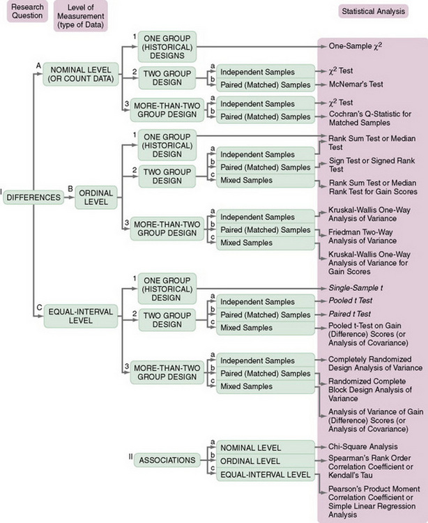
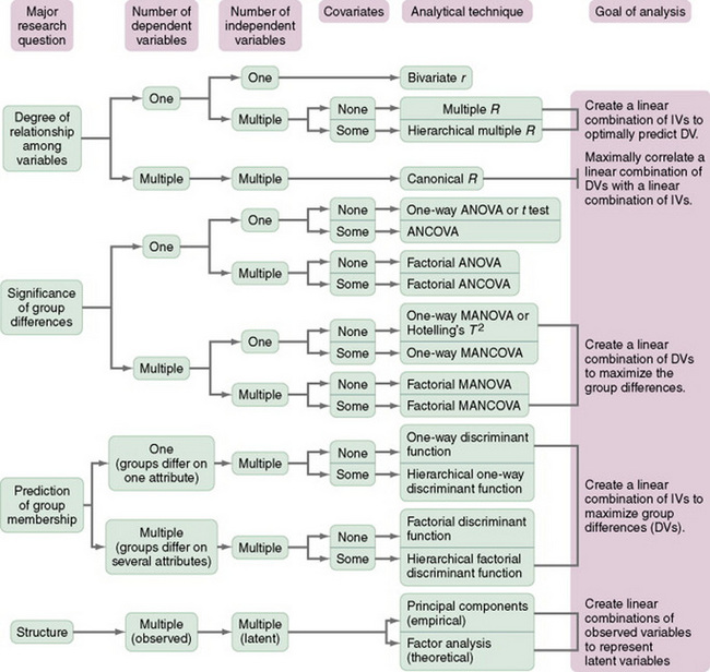
One disadvantage of decision trees is that if you make an incorrect or uninformed decision (guess), you can be led down a path in which you might select an inappropriate statistical procedure for your study. Decision trees are often constrained by space and therefore do not include all the information needed to make an appropriate selection. The most extensive decision tree that we have found is presented in A Guide for Selecting Statistical Techniques for Analyzing Social Science Data by Andrews, Klem, Davidson, O’Malley, and Rodgers (1981). The following examples of questions designed to guide the selection or evaluation of statistical procedures were extracted from this book:
13. Do you want to treat the ordinal variable as though it were based on an underlying normally distributed interval variable?
15. Do you want a measure of the strength of the relationship between the variables or a test of the statistical significance of differences between groups (Kenny, 1979)?
16. Are you willing to assume that an intervally scaled variable is normally distributed in the population?
18. Do you want to statistically remove the linear effects of one or more covariates from the dependent variable?
21. Do you want to find clusters of variables that are more strongly related to one another than to the remaining variables?
Each question confronts you with a decision. The decision you make narrows the field of available statistical procedures. Decisions must be made regarding the following:
1. Number of variables (1, 2, more than 2)
2. Type of measurement (nominal, ordinal, interval)
3. Type of variable (independent, dependent, research)
4. Distribution of variable (normal, non-normal)
5. Type of relationship (linear, nonlinear)
6. What you want to measure (strength of relationship, difference between groups)
7. Nature of the groups (equal or unequal in size, matched or unmatched, dependent or independent)
8. Type of analysis (descriptive, classification, methodological, relational, comparison, predicting outcomes, intervention testing, causal modeling, examining changes across time)
As you can see, selecting and evaluating statistical procedures requires that you make a number of judgments regarding the nature of the data and what you want to know. Knowledge of the statistical procedures and their assumptions is necessary for selecting appropriate procedures. You must weigh the advantages and disadvantages of various statistical options. Access to a statistician can be invaluable in selecting the appropriate procedures.
SUMMARY
• This chapter introduces you to the concepts of statistical theory and discusses some of the more pragmatic aspects of quantitative data analysis: the purposes of statistical analysis, the process of performing data analysis, the choice of the appropriate statistical procedures for a study, and resources for statistical analysis.
• Two types of errors can occur when making decisions about the meaning of a value obtained from a statistical test: type I errors and type II errors.
• A type I error occurs when the researcher concludes that the samples tested are from different populations (the difference between groups is significant) when, in fact, the samples are from the same population (no significant difference between groups).
• A type II error occurs when the researcher concludes that the samples are from the same population when, in fact, they are from different populations.
• The formal definition of the level of significance, or alpha (α), is the probability of making a type I error when the null hypothesis is true.
• The level of significance, developed from decision theory, is the cutoff point used to determine whether the samples being tested are members of the same population or from different populations.
• Power is the probability that a statistical test will detect a significant difference that exists.
• Statistics can be used for a variety of purposes, such as to (1) summarize, (2) explore the meaning of deviations in the data, (3) compare or contrast descriptively, (4) test the proposed relationships in a theoretical model, (5) infer that the findings from the sample are indicative of the entire population, (6) examine causality, (7) predict, or (8) infer from the sample to a theoretical model.
• Quantitative data analysis consists of several stages: (1) preparation of the data for analysis; (2) description of the sample; (3) testing the reliability of measurement; (4) exploratory analysis of the data; (5) confirmatory analysis guided by the hypotheses, questions, or objectives; and (6) post hoc analysis.
REFERENCES
Andrews, F.M., Klem, L., Davidson, T.N., O’Malley, P.M., Rodgers, W.L. A guide for selecting statistical techniques for analyzing social science data, 2nd ed. Ann Arbor, MI: Survey Research Center, Institute for Social Research, University of Michigan, 1981.
Barnett, V. Comparative statistical inference. New York: Wiley, 1982.
Box, G.E.P., Hunter, W.G., Hunter, J.S. Statistics for experimenters. New York: Wiley, 1978.
Brent, E.E., Jr., Scott, J.K., Spencer, J.C. Ex-Sample: An expert system to assist in designing sampling plans. User’s guide and reference manual. Columbia, MO: Idea Works, 1988. [Version 2.0].
Chervany, N.L. The logic and practice of statistics. Bloomington, MN: Written materials provided with a presentation at the Institute of Management Science, 1977. [December 15].
Cohen, J. Statistical power analysis for the behavioral sciences, (2nd ed.). New York: Academic Press, 1988.
Conover, W.J. Practical nonparametric statistics. New York: Wiley, 1971.
Cox, D.R. Planning of experiments. New York: Wiley, 1958.
Glass, G.V., Stanley, J.C. Statistical methods in education and psychology. Englewood Cliffs, NJ: Prentice-Hall, 1970.
Good, I.J. Good thinking: The foundations of probability and its applications. Minneapolis: University of Minnesota Press, 1983.
Hinshaw, A.S., Schepp, K. Problems in doing nursing research: How to recognize garbage when you see it. Western Journal of Nursing Research. 1984;6(1):126–130.
Kenny, D.A. Correlation and causality. New York: Wiley, 1979.
Roscoe, J.T. Fundamental research statistics for the behavioral sciences. New York: Holt, Rinehart & Winston, 1969.
Slakter, M.J., Wu, Y.B., Suzuki-Slakter, N.S. *, **, and ***, statistical nonsense at the .00000 level. Nursing Research. 1991;40(4):248–249.
Tukey, J.W. Exploratory data analysis. Reading, MA: Addison-Wesley, 1977.
Volicer, B.J. Multivariate statistics for nursing research. New York: Grune & Stratton, 1984.
Yarandi, H.N. Using the SAS system to estimate sample size and power for comparing two binomial proportions. Nursing Research. 1994;43(2):124–125.