Examples

Mathematical statement. A linear function describes a change in one variable (dependent or y variable) that is directly proportional to another variable (independent or x variable). There may or may not be a constant factor which is equal to y when x is zero. Thus:

where a is the slope of the line and b is the constant factor. In any one particular relationship a and b are assumed to be constant but both may have different values under other circumstances. There are not therefore true constants (like π, for example) and are more precisely termed parameters, whilst y and x are variables.

Graphical representation. Figure E.1 shows a plot of a linear function following the convention that the independent variable (x) is plotted on the abscissa and the dependent variable (y) on the ordinate. Note that the relationship is a straight line and simple regression analysis is based on the assumption that the relationship is of this type. If the slope (a) is positive, the line goes upwards and to the right. If the slope is negative, the line goes upwards and to the left.

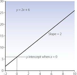
Figure E.1 A linear function plotted on linear coordinates. Examples include pressure/flow rate relationships with laminar flow (see Figure 4.2) and Pco₂/ventilation response curves (see Figure 5.5).

Examples

Mathematical statement. A rectangular hyperbola describes a relationship when the dependent variable y is inversely proportional to the independent variable x thus:

The asymptote of x is its value when y is infinity and the asymptote of y is its value when x is infinity. If b is zero, then the relationship may be simply represented as follows:

Graphical representation. Figure E.2A shows rectangular hyperbolas with and without constant factors. Changes in the value of a alter the curvature but not the asymptotes. Figure E.2B shows the same relationships plotted on logarithmic coordinates. The relationship is now linear but with a negative slope of unity because, if:

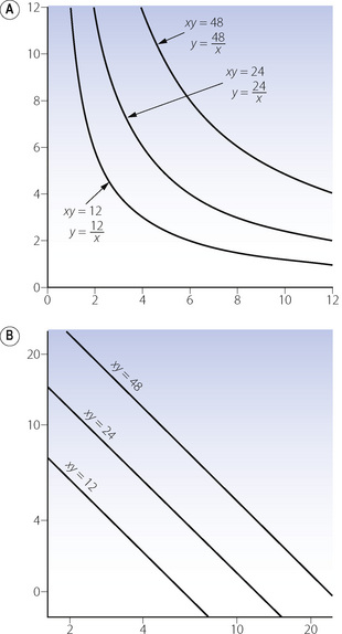
Figure E.2 Rectangular hyperbolas plotted on (A) linear coordinates and (B) logarithmic coordinates. Examples include the relationships between alveolar gas tensions and alveolar ventilation (see Figures 10.9, 11.2), Po₂/ventilation response curves (see Figure 5.8) and the relationship between airway resistance and lung volume (see Figures 4.5 and 22.13).

then:

Example

With fully turbulent gas flow, pressure gradient changes according to the square of gas flow and the plot is a typical parabola (Chapter 4).

Mathematical statement. A parabola is described when the dependent variable (y) changes in proportion to the square of the independent variable (x), thus:

Graphical representation. On linear coordinates, a parabola, with positive values of the abscissa, shows a steeply rising curve (Figure E.3A), which may be confused with an exponential function (see below) although it is fundamentally different. On logarithmic coordinates for both abscissa and ordinate, a parabola becomes a straight line with a slope of two (Figure E.3B) because log y = log a + 2 log x (a and log a are parameters).

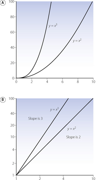
Figure E.3 Parabolas plotted on (A) linear coordinates and (B) logarithmic coordinates. An example is the pressure/volume relationship with turbulent flow (see Figure 4.3B).

General Statement

An exponential function describes a change in which the rate of change of the dependent variable is proportional to the magnitude of the independent variable at that time. Thus, the rate of change of y with respect to x (i.e. dy/dx)^* varies in proportion to the value of y at that instant. That is to say:

where k is a constant or a parameter.

This general equation appears with minor modifications in three main forms. To the biological worker they may be conveniently described as the tear-away, the wash-out and the wash-in.

The Tear-away Exponential Function

This must be described first, as it is the simplest form of the exponential function. It is, however, the least important of the three in relation to respiratory function.

Simple statement. In a tear-away exponential function, the quantity under consideration increases at a rate which is in direct proportion to its actual value – the richer one is, the faster one makes money.

Examples. Classic examples are compound interest, and the mythical water-lily that doubles its diameter every day (Figure E.4). A typical biological example is the free spread of a bacterial colony in which (for example) each bacterium divides every 20 minutes. The doubling time of this example would be 20 minutes.

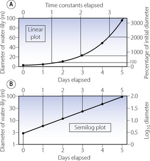
Figure E.4 The growth of a water-lily that doubles its diameter every day – a typical tear-away exponential function. Initial diameter, 3 metres; size doubled every day (i.e. doubling time = 1 day).

Mathematical statement. In the case of exponential functions relevant to respiratory function, the independent variable x almost invariably represents time, and so we shall take the liberty of replacing x with t throughout. The tear-away function may thus be represented as follows:

A little mathematical processing will convert this equation into a more useful form, which will indicate the instantaneous value of y at any time, t.

First multiply both sides by dt/y:

Next integrate both sides with respect to t:

(C₁ and C₂ are constants of integration and may be collected on the right-hand side.)

Finally, take antilogs of each side to the base e:

At zero time, t = 0 and e^kt = 1. Therefore the constant e^{(C2 − C1)} equals the initial value of y, which we may call y₀. Our final equation is thus:

y₀ is the initial value of the variable y at zero time.

e is the base of natural logarithms. This constant (2.71828…) possesses many remarkable mathematical properties.

k is a constant that defines the speed of the particular function. For example, it will differ by a factor of two if our mythical water-lily doubles its size every 12 hours instead of every day. In the case of the wash-out and wash-in, we shall see that k is directly related to certain important physiological quantities, from which we may predict the speed of certain biological changes.

Instead of using e, it is possible to take logs to the more familiar base 10, thus:

This is a perfectly valid way of expressing a tear-away exponential function, but you will notice that the constant k has changed to k₁. This new constant does not have the simple relationships of physiological variables mentioned above. It does, however, bear a constant relationship to k, as follows:

Graphical representation. On linear graph paper, a tear-away exponential function rapidly disappears off the top of the paper (Figure E.4). If plotted on semi-logarithmic paper (time on a linear axis and y on a logarithmic axis), the plot becomes a straight line and this is a most convenient method of presenting such a function. The logarithmic plots in Figures E.4-E.6 are all plotted on semi-log paper.

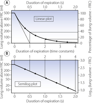
Figure E.5 Passive expiration – a typical wash-out exponential function. Tidal volume, 500 ml; compliance, 0.5 l.kPa⁻¹ (50 ml.cmH₂O⁻¹); airway resistance, 1 kPa.l⁻¹.s (10 cmH₂O.l⁻¹.s); time constant, 0.5 s; half-life, 0.35 s. The point on the curve indicate the passage of successive half-lives. Note that the logarithmic coordinate has no zero. This accords with the lung volume approaching, but never actually equalling, the FRC.

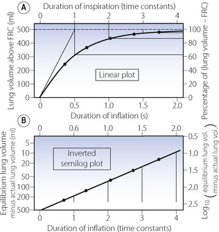
Figure E.6 Passive inflation of the lungs with a sustained mouth pressure – a typical wash-in exponential function. Final tidal volume, 500 ml; compliance, 0.5 l.kPa⁻¹ (50 ml.cmH₂O⁻¹); airway resistance, 1 kPa.l⁻¹.s (10 cmH₂O.l⁻¹.s); time constant, 0.5 s; half-life, 0.35 s. The points on the curves indicate the passage of successive half-lives. Note that, for the semilog plot, the log scale (ordinate) is from above downwards and indicates the difference between the equilibrium lung volume (inflation pressure maintained indefinitely) and the actual lung volume.

The Wash-out Or Die-away Exponential Function

The account of the tear-away exponential function has really been an essential introduction to the wash-out or die-away exponential function, which is of great importance to the biologist in general, and the respiratory physiologist in particular.

Simple statement. In a wash-out exponential function, the quantity under consideration falls at a rate which decreases progressively in proportion to the distance it still has to fall. It approaches but, in theory, never reaches zero.

Examples. Familiar examples are cooling curves, radioactive decay and water running out of the bath. In the last example the rate of flow of bath water to waste is proportional to the pressure of water, which is proportional to the depth of water in the bath, which in turn is proportional to the quantity of water in the bath (assuming that the sides are vertical). Therefore, the flow rate of water to waste is proportional to the amount of water left in the bath, and decreases as the bath empties. The last molecule of bath water takes an infinitely long time to drain away.

In the field of respiratory physiology, examples include:

Mathematical statement. When a quantity decreases with time, the rate of change is negative. Therefore, the wash-out exponential function is written thus:

from which we may derive the following equations, which give the value of y at any time t:

which is simply another way of saying:

y₀ is again the initial value of y at zero time. In Figure E.5, y₀ is the initial value of (lung volume − FRC) at the start of expiration; that is to say, the tidal volume inspired.

e is again the base of natural logarithms (2.718 28…).

k is the constant that defines the rate of decay, and is the reciprocal of a most important quantity known as the time constant, represented by the Greek letter tau (τ). Three things should be known about the time constant:

We may now consider the example of passive expiration. Let V represent the lung volume (above FRC), then −dV/dt is the instantaneous expiratory gas flow rate. Assuming Poiseuille’s law is obeyed:

when P is the instantaneous alveolar-to-mouth pressure gradient and R is the airway resistance. However, compliance (C) = V/P. Therefore:

or:

Then by integration and taking antilogs as described above:

By analogy with the general equation of the wash-out exponential function, it is clear that CR = 1/k = τ (the time constant). Thus the time constant equals the product of compliance and resistance.^†

^† It is strange at first sight that two quantities as complex as compliance and resistance should have a product as simple as time. In fact, the MLT units (Appendix A) check perfectly well:

This is analogous to the discharge of an electrical capacitor through a resistance, when the time constant of discharge equals the product of the capacitance and the resistance.

Half-life. It is often convenient to use the half-life instead of the time constant. This is the time required for y to change to half of its previous value. The special attraction of the half-life is its ease of measurement. The half-life of a radioactive element may be determined quite simply. First of all the degree of activity is measured and the time noted. Its activity is then followed and the time noted at which its activity is exactly half the initial value. The difference between the two times is the half-life and is constant at all levels of activity. Half-lives are shown in Figures E.4-E.6 as dots on the curves. For a particular exponential function there is a constant relationship between the time constant and the half-life.

Graphical representation. Plotting a wash-out exponential function is similar to the tear-away function (Figure E.5). A semi-log plot is particularly convenient as the curve (being straight) may then be defined by far fewer observations. It is also easy to extrapolate backwards to zero time if the initial value is required but could not be measured directly for some reason. It is, for example, an essential step in the measurement of cardiac output with a dye that is rapidly lost from the circulation (page 115).

The Wash-in Exponential Function

The wash-in function is also of special importance to the respiratory physiologist and is the mirror image of the wash-out function.

Simple statement. In a wash-in exponential function, the quantity under consideration rises towards a limiting value, at a rate that decreases progressively in proportion to the distance it still has to rise.

Examples. A typical example would be a mountaineer who each day manages to climb half the remaining distance between his overnight camp and the summit of the mountain. His rate of ascent declines exponentially and he will never reach the summit. A graph of his altitude plotted against time would resemble a ‘wash-in’ curve.

Biological examples include the reverse of those listed for the wash-out function:

Mathematical statement. With a wash-in exponential function, y increases with time and therefore the rate of change is positive. As time advances, the rate of change falls towards zero. The initial value of y is often zero and y approaches a final limiting value that we may designate y_∞ – that is the value of y when time is infinity (∞). A change of this type is indicated thus:

As y approaches y_∞ so the quantity within the parentheses approaches zero, and the rate of change slows down. The corresponding equation that indicates the instantaneous value of y is:

y_∞ is the limiting value of y (attained only at infinite time).

e is again the base of natural logarithms.

k is a constant defining the rate of build-up and, as is the case of the wash-out function, it is the reciprocal of the time constant the significance of which is described above. It is the time that would be required to reach completion, if the initial rate of change were maintained without slowing down.

After 1 time constant, y will have risen to approximately 100 − 37 = 63% of its final value.

After 2 time constants, y will have risen to approximately 100 − 13.5 = 86.5% of its final value.

After 3 time constants, y will have risen to approximately 100 − 5 = 95% of its final value.

After 5 time constants, y will have risen to approximately 100 − 1 = 99% of its final value.

As in the wash-out function representing passive exhalation, the time constant for the corresponding wash-in exponential function (passive inflation of the lungs) equals the product of compliance and resistance. For the wash-in of a substance into an organ, the time constant equals tissue volume divided by blood flow, or FRC divided by alveolar ventilation as the case may be. As above, the time constant is approximately 1.5 times the half-life.

There are many situations in which the same parameters apply to both wash-in and wash-out functions of the same system. The time constant for each function will then be the same. A classic example is the charging of an electrical capacitor through a resistance, and then allowing it to discharge to earth through the same resistor. The time constant is the same for each process and equals the product of capacitance and resistance. This is approximately true for passive deflation and inflation of the lungs (Figures E.5 and E.6), on the assumption that compliance and airway resistance remain the same.

Graphical representation. The wash-in function may be represented on linear paper as for the other types of exponential function. However, for the semi-log plot, the paper must be turned upside down and the plot made as indicated in Figure E.6. The curve will then be a straight line.