10 Pharmacokinetics
Overview
We explain the importance of pharmacokinetic analysis and present a simple approach to this. We explain how drug clearance determines the steady-state plasma concentration during constant-rate drug administration and how the characteristics of absorption and distribution (considered in Ch. 8) plus metabolism and excretion (considered in Ch. 9) determine the time course of drug concentration in blood plasma during and following drug administration. The effect of different dosing regimens on the time course of drug concentration in plasma is explained. Population pharmacokinetics is mentioned briefly, and a final section considers limitations to the pharmacokinetic approach.
Introduction: Definition and Uses of Pharmacokinetics
Pharmacokinetics may be defined as the measurement and formal interpretation of changes with time of drug concentrations in one or more different regions of the body in relation to dosing (‘what the body does to the drug’). This distinguishes it from pharmacodynamics (‘what the drug does to the body’, i.e. events consequent on interaction of the drug with its receptor or other primary site of action). The distinction is useful, although the words cause dismay to etymological purists. ‘Pharmacodynamic’ received an entry in a dictionary of 1890 (’relating to the powers or effects of drugs’) whereas pharmacokinetic studies only became possible with the development of sensitive, specific and accurate physicochemical analytical techniques, especially chromatography and mass spectrometry, for measuring drug concentrations in biological fluids in the latter part of the 20th century. The time course of drug concentration following dosing depends on the processes of absorption, distribution, metabolism and excretion that we have considered qualitatively in Chapters 8 and 9.
In practice, pharmacokinetics usually focuses on concentrations of drug in blood plasma, which is easily sampled via venepuncture, since plasma concentrations are assumed usually to bear a clear relation to the concentration of drug in extracellular fluid surrounding cells that express the receptors or other targets with which drug molecules combine. This underpins what is termed the target concentration strategy. Individual variation (Ch. 56) in response to a given dose of a drug is often greater than variability in the plasma concentration at that dose. Plasma concentrations (Cp) are therefore useful in the early stages of drug development (see below), and in the case of a few drugs plasma drug concentrations are also used in routine clinical practice to individualise dosage so as to achieve the desired therapeutic effect while minimising adverse effects in each individual patient, an approach known as therapeutic drug monitoring (often abbreviated TDM—see Table 10.1 for examples of some drugs where a therapeutic range of plasma concentrations has been established). Concentrations of drug in other body fluids (e.g. urine,1 saliva, cerebrospinal fluid, milk) may add useful information in some special situations.
Table 10.1 Examples of drugs where therapeutic drug monitoring (TDM) of plasma concentrations is used clinically
| Category | Example(s) | See Chapter |
|---|---|---|
| Immunosuppressants | Ciclosporine, tacrolimus | 26 |
| Cardiovascular | Digoxin | 21 |
| Respiratory | Theophylline | 16, 27 |
| CNS | Lithium, several antiepileptic drugs | 46, 44 |
| Antibacterials | Aminoglycosides | 50 |
| Antineoplastics | Methotrexate | 55 |
Formal interpretation of pharmacokinetic data consists of fitting concentration versus time data to a theoretical model and determining parameters that describe the observed behaviour. The parameters can then be used to adjust the dose regimen to achieve a desired target plasma concentration estimated initially from pharmacological experiments on cells, tissues or laboratory animals, and modified in light of the human pharmacology if necessary. Some descriptive pharmacokinetic characteristics can be observed directly by inspecting the time course of drug concentration in plasma following dosing—important examples2 are the maximum plasma concentration following a given dose of a drug administered in a defined dosing form (Cmax) and the time (Tmax) between drug administration and achieving Cmax. Other pharmacokinetic parameters are estimated mathematically from experimental data; examples include volume of distribution (Vd) and clearance (CL), concepts that have been introduced in Chapters 8 and 9 respectively and to which we return below.
Uses of Pharmacokinetics
Knowledge of pharmacokinetics is crucial in drug development, both to make sense of preclinical toxicity testing and of whole animal pharmacology,3 and to decide on an appropriate dosing regimen for clinical studies of efficacy (see Ch. 60). Drug regulators need detailed pharmacokinetic information for the same reasons, and must understand principles of bioavailability and bioequivalence (Ch. 8) to make decisions about licensing generic versions of drugs as these lose their patent protection. An understanding of the general principles of pharmacokinetics is important for clinicians, who need to understand how dosage recommendations in the product information provided with licensed drugs have been arrived at if they are to use the drug optimally. Clinicians also need to understand the principles of pharmacokinetics if they are to identify and evaluate possible drug interactions (see Ch. 56). They also need to be able to interpret drug concentrations for TDM and to adjust dose regimens rationally. In particular, clinicians dealing with a severely ill patient often need to individualise the dose regimen depending on the urgency of achieving a therapeutic plasma concentration, and whether the clearance of the drug is impaired because of renal or liver disease.
Scope of this Chapter
The objectives of this chapter are to familiarise the reader with the meanings of important pharmacokinetic parameters; to explain how the total clearance of a drug determines its steady-state plasma concentration during continuous administration; to present a simple model in which the body is represented as a single well-stirred compartment, of volume Vd, that describes the situation before steady state is reached in terms of elimination half-life (t1/2); to consider some situations where the simple model is inadequate, and either a two-compartment model or a model where clearance varies with drug concentration (‘non-linear kinetics’) is needed; to mention briefly the field of population kinetics; and finally to consider some of the limitations inherent in the pharmacokinetic approach. More detailed accounts are provided by Atkinson et al. (2002), Birkett (2002), Jambhekar & Breen (2009) and Rowland & Tozer (2010).
Drug Elimination Expressed as Clearance
The concept of clearance was introduced in 1929 as a means of expressing the rate of urea excretion in adult humans, in terms of the volume of blood cleared of urea in 1 minute. Clearance of a drug can be defined analogously as the volume of plasma from which all the drug molecules would need to be removed per unit time to achieve the overall rate of elimination of drug from the body. Subsequently, as mentioned in Chapter 9, creatinine rather than urea clearance has become the routine clinical measure of renal functional status because it more closely reflects the glomerular filtration rate. Van Slyke introduced the equation given in Chapter 9 for estimating renal clearance (CLren). This follows from the law of conservation of mass, and is written:
where Cu is the urine concentration of the substance of interest (whether endogenous such as urea or creatinine, or exogenous as in the case of an administered drug), Cp its concentration in plasma and Vu the urine flow rate in units of volume/time. Cu and Cp are expressed in the same units of mass/unit volume (e.g. mg/l) so their units cancel out and CLren has the same units as V, namely volume/unit time—e.g. ml/min or l/h.
The overall clearance of a drug (CLtot) is the fundamental pharmacokinetic parameter describing drug elimination. It is defined as the volume of plasma containing the total amount of drug that is removed from the body in unit time by all routes. Overall clearance is the sum of clearance rates for each mechanism involved in eliminating the drug, usually renal clearance (CLren) and metabolic clearance (CLmet) plus any additional appreciable routes of elimination (faeces, breath, etc.). It relates the rate of elimination of a drug (in units of mass/unit time) to Cp:

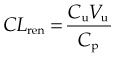
Drug clearance can be determined in an individual subject by measuring the plasma concentration of the drug (in units of, say, mg/l) at intervals during a constant-rate intravenous infusion (delivering, say, X mg of drug per h), until a steady state is approximated (Fig. 10.1A). At steady state, the rate of input to the body is equal to the rate of elimination, so:
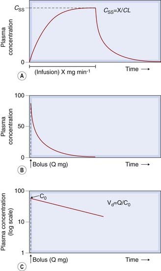
Fig. 10.1 Plasma drug concentration-time curves. [A] During a constant intravenous infusion at rate X mg/min, indicated by the horizontal bar, the plasma concentration (C) increases from zero to a steady-state value (CSS); when the infusion is stopped, C declines to zero. [B] Following an intravenous bolus dose (Q mg), the plasma concentration rises abruptly and then declines towards zero. [C] Data from panel B plotted with plasma concentrations on a logarithmic scale. The straight line shows that concentration declines exponentially. Extrapolation back to the ordinate at zero time gives an estimate of C0, the concentration at zero time, and hence of Vd, the volume of distribution.

where CSS is the plasma concentration at steady state, and CLtot is in units of volume/time (l/h in the example given).
For many drugs, clearance in an individual subject is the same at different doses (at least within the range of doses used therapeutically—but see the section on saturation kinetics below for exceptions), so knowing the clearance enables one to calculate the dose rate needed to achieve a desired steady-state (’target’) plasma concentration from equation 10.3.
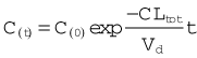
CLtot can also be estimated by measuring plasma concentrations at intervals following a single intravenous bolus dose of, say, Q mg (Fig. 10.1B):
where AUC0–∞ is the area under the full curve4 relating Cp to time following a bolus dose given at time t = 0. (See Ch. 8, and Birkett, 2002, for a fuller account of AUC0–∞.)
Note that these estimates of CLtot, unlike estimates based on the rate constant or half-life (see below), do not depend on any particular compartmental model.
Single-Compartment Model
Consider a highly simplified model of a human being, which consists of a single well-stirred compartment, of volume Vd (distribution volume), into which a quantity of drug Q is introduced rapidly by intravenous injection, and from which it can escape either by being metabolised or by being excreted (Fig. 10.2). For most drugs, Vd is an apparent volume rather than the volume of an anatomical compartment. It links the total amount of drug in the body to its concentration in plasma (see Ch. 8). The quantity of drug in the body when it is administered as a single bolus is equal to the administered dose Q. The initial concentration, C0, will therefore be given by:
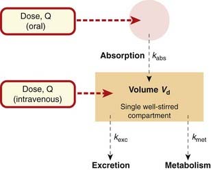
Fig. 10.2 Single-compartment pharmacokinetic model.
This model is applicable if the plasma concentration falls exponentially after drug administration (as in Fig. 10.1).

In practice, C0 is estimated by extrapolating the linear portion of a semilogarithmic plot of Cp against time back to its intercept at time 0 (Fig. 10.1C). Cp at any time depends on the rate of elimination of the drug (i.e. on its total clearance, CLtot) as well as on the dose and Vd. Many drugs exhibit first-order kinetics where the rate of elimination is directly proportional to drug concentration. Drug concentration then decays exponentially (Fig. 10.3), being described by the equation:
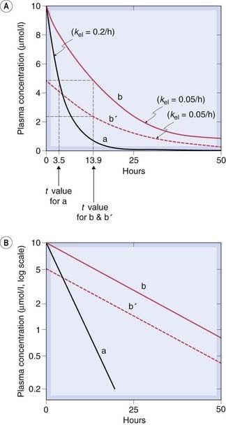
Fig. 10.3 Predicted behaviour of single-compartment model following intravenous drug administration at time 0.
Drugs a and b differ only in their elimination rate constant, kel. Curve b′ shows the plasma concentration time course for a smaller dose of b. Note that the half-life (t1/2) (indicated by broken lines) does not depend on the dose. [A] Linear concentration scale. [B] Logarithmic concentration scale.
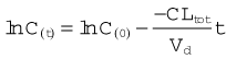
Plotting Ct on a logarithmic scale against t (on a linear scale) yields a straight line with slope −CLtot/Vd. The inverse of this slope (CLtot/Vd) is the elimination rate constant kel, which has units of (time)−1. It represents the fraction of drug in the body eliminated per unit of time. For example, if the rate constant is 0.1 h−1 this implies that one-tenth of the drug remaining in the body is eliminated each hour.
The elimination half-life, t1/2, is an easily conceptualised parameter inversely related to kel. It is the time taken for Cp to decrease by 50%, and is equal to ln2/kel (= 0.693/kel). The plasma half-life is therefore determined by Vd as well as by CLtot. It enables one to predict what will happen after drug administration is initiated before steady state is reached, and after drug administration has been stopped while Cp declines toward zero.
When the single-compartment model is applicable, the drug concentration in plasma approaches the steady-state value approximately exponentially during a constant infusion (Fig. 10.1A). When the infusion is discontinued, the concentration falls exponentially towards zero: after one half-life, the concentration will have fallen to half the initial concentration; after two half-lives, it will have fallen to one-quarter the initial concentration; after three half-lives, to one-eighth; and so on. It is intuitively obvious that the longer the half-life, the longer the drug will persist in the body after dosing is discontinued. It is less obvious, but nonetheless true, that during chronic drug administration the longer the half-life, the longer it will take for the drug to accumulate to its steady-state level: one half-life to reach 50% of the steady-state value, two to reach 75%, three to reach 87.5% and so on. This is extremely helpful to a clinician deciding how to start treatment. If the drug in question has a half-life of approximately 24 h, for example, it will take 3–5 days to approximate the steady-state concentration during a constant-rate infusion. If this is too slow in the face of the prevailing clinical situation, a loading dose may be used in order to achieve a therapeutic concentration of drug in the plasma more rapidly (see below). The size of such a dose is determined by the volume of distribution (equation 10.6).
Effect of Repeated Dosing
Drugs are usually given as repeated doses rather than single injections or a constant infusion. Repeated injections (each of dose Q) give a more complicated pattern than the smooth exponential rise during intravenous infusion, but the principle is the same (Fig. 10.4). The concentration will rise to a mean steady-state concentration with an approximately exponential time course, but will oscillate (through a range Q/Vd). The smaller and more frequent the doses, the more closely the situation approaches that of a continuous infusion, and the smaller the swings in concentration. The exact dosage schedule, however, does not affect the mean steady-state concentration, or the rate at which it is approached. In practice, a steady state is effectively achieved after three to five half-lives. Speedier attainment of the steady state can be achieved by starting with a larger dose, as mentioned above. Such a loading dose is sometimes used when starting treatment with a drug with a half-life that is long in the context of the urgency of the clinical situation, as may be the case when treating cardiac dysrhythmias with drugs such as amiodarone or digoxin (Ch. 21) or initiating anticoagulation with heparin (Ch. 24).
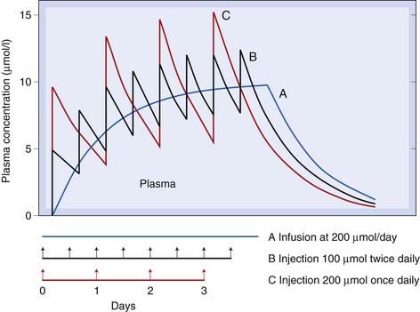
Fig. 10.4 Predicted behaviour of single-compartment model with continuous or intermittent drug administration.
Smooth curve A shows the effect of continuous infusion for 4 days; curve B the same total amount of drug given in eight equal doses; and curve C the same total amount of drug given in four equal doses. The drug has a half-life of 17 h and a volume of distribution of 20 l. Note that in each case a steady state is effectively reached after about 2 days (about three half-lives), and that the mean concentration reached in the steady state is the same for all three schedules.
Effect of Variation in Rate of Absorption
If a drug is absorbed slowly from the gut or from an injection site into the plasma, it is (in terms of a compartmental model) as though it were being slowly infused at a variable rate into the bloodstream. For the purpose of kinetic modelling, the transfer of drug from the site of administration to the central compartment can be represented approximately by a rate constant, kabs (see Fig. 10.2). This assumes that the rate of absorption is directly proportional, at any moment, to the amount of drug still unabsorbed, which is at best a rough approximation to reality. The effect of slow absorption on the time course of the rise and fall of the plasma concentration is shown in Figure 10.5. The curves show the effect of spreading out the absorption of the same total amount of drug over different times. In each case, the drug is absorbed completely, but the peak concentration appears later and is lower and less sharp if absorption is slow. In the limiting case, a dosage form that releases drug at a constant rate as it traverses the ileum (Ch. 8) approximates a constant-rate infusion. Once absorption is complete, the plasma concentration declines with the same half-time, irrespective of the rate of absorption.
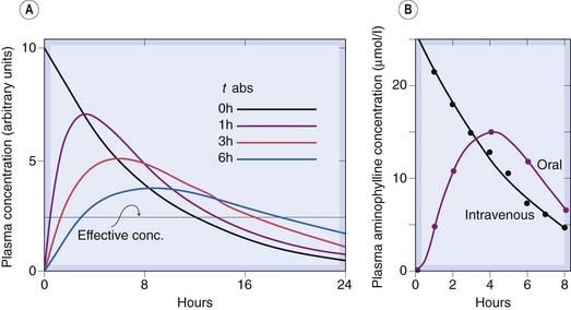
Fig. 10.5 The effect of slow drug absorption on plasma drug concentration.
[A] Predicted behaviour of single-compartment model with drug absorbed at different rates from the gut or an injection site. The elimination half-time is 6 h. The absorption half-times (t1/2 abs) are marked on the diagram. (Zero indicates instantaneous absorption, corresponding to intravenous administration.) Note that the peak plasma concentration is reduced and delayed by slow absorption, and the duration of action is somewhat increased. [B] Measurements of plasma aminophylline concentration in humans following equal oral and intravenous doses.
(Data from Swintowsky J V 1956 J Am Pharm Assoc 49: 395.)
 For the kind of pharmacokinetic model discussed here, the area under the plasma concentration–time curve (AUC) is directly proportional to the total amount of drug introduced into the plasma compartment, irrespective of the rate at which it enters. Incomplete absorption, or destruction by first-pass metabolism before the drug reaches the plasma compartment, reduces AUC after oral administration (see Ch. 8). Changes in the rate of absorption, however, do not affect AUC. Again, it is worth noting that provided absorption is complete, the relation between the rate of administration and the steady-state plasma concentration (equation 10.4) is unaffected by kabs, although the size of the oscillation of plasma concentration with each dose is reduced if absorption is slowed.
More Complicated Kinetic Models
So far, we have considered a single-compartment pharmacokinetic model in which the rates of absorption, metabolism and excretion are all assumed to be directly proportional to the concentration of drug in the compartment from which transfer is occurring. This is a useful way to illustrate some basic principles but is clearly a physiological oversimplification. The characteristics of different parts of the body, such as brain, body fat and muscle, are quite different in terms of their blood supply, partition coefficient for drugs and the permeability of their capillaries to drugs. These differences, which the single-compartment model ignores, can markedly affect the time courses of drug distribution and action, and much theoretical work has gone into the mathematical analysis of more complex models (see Atkinson et al., 2002; Rowland & Tozer, 2010). They are beyond the scope of this book, and perhaps also beyond the limit of what is actually useful, for the experimental data on pharmacokinetic properties of drugs are seldom accurate or reproducible enough to enable complex models to be tested critically.
The two-compartment model, which introduces a separate ‘peripheral’ compartment to represent the tissues, in communication with the ‘central’ plasma compartment, more closely resembles the real situation without involving excessive complications.
Two-Compartment Model
The two-compartment model is a widely used approximation in which the tissues are lumped together as a peripheral compartment. Drug molecules can enter and leave the peripheral compartment only via the central compartment (Fig. 10.6), which usually represents the plasma (or plasma plus some extravascular space in the case of a few drugs that distribute especially rapidly). The effect of adding a second compartment to the model is to introduce a second exponential component into the predicted time course of the plasma concentration, so that it comprises a fast and a slow phase. This pattern is often found experimentally, and is most clearly revealed when the concentration data are plotted semilogarithmically (Fig. 10.7). If, as is often the case, the transfer of drug between the central and peripheral compartments is relatively fast compared with the rate of elimination, then the fast phase (often called the α phase) can be taken to represent the redistribution of the drug (i.e. drug molecules passing from plasma to tissues, thereby rapidly lowering the plasma concentration). The plasma concentration reached when the fast phase is complete, but before appreciable elimination has occurred, allows a measure of the combined distribution volumes of the two compartments; the half-time for the slow phase (the β phase) provides an estimate of kel. If a drug is rapidly metabolised, the α and β phases are not well separated, and the calculation of Vd and kel is not straightforward. Problems also arise with drugs (e.g. very fat-soluble drugs) for which it is unrealistic to lump all the peripheral tissues together.

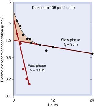
Fig. 10.7 Kinetics of diazepam elimination in humans following a single oral dose.
The graph shows a semilogarithmic plot of plasma concentration versus time. The experimental data (black symbols) follow a curve that becomes linear after about 8 h (slow phase). Plotting the deviation of the early points (pink shaded area) from this line on the same coordinates (red symbols) reveals the fast phase. This type of two-component decay is consistent with the two-compartment model (Fig. 10.6) and is obtained with many drugs.
(Data from Curry S H 1980 Drug disposition and pharmacokinetics. Blackwell, Oxford.)
Saturation Kinetics
In a few cases, such as ethanol, phenytoin and salicylate, the time course of disappearance of drug from the plasma does not follow the exponential or biexponential patterns shown in Figures 10.3 and 10.7 but is initially linear (i.e. drug is removed at a constant rate that is independent of plasma concentration). This is often called zero-order kinetics to distinguish it from the usual first-order kinetics that we have considered so far (these terms have their origin in chemical kinetic theory). Saturation kinetics is a better term. Figure 10.8 shows the example of ethanol. It can be seen that the rate of disappearance of ethanol from the plasma is constant at approximately 4 mmol/l per h, irrespective of dose or of the plasma concentration of ethanol. The explanation for this is that the rate of oxidation by the enzyme alcohol dehydrogenase reaches a maximum at low ethanol concentrations, because of limited availability of the cofactor NAD+ (see Ch. 48, Fig. 48.5).
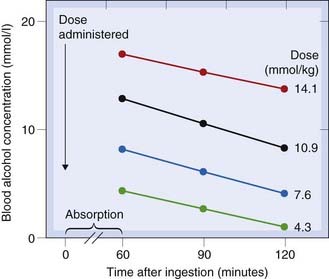
Fig. 10.8 Saturating kinetics of alcohol elimination in humans.
The blood alcohol concentration falls linearly rather than exponentially, and the rate of fall does not vary with dose.
(From Drew G C et al. 1958 Br Med J 2: 5103.)
Saturation kinetics has several important consequences (see Fig. 10.9). One is that the duration of action is more strongly dependent on dose than is the case with drugs that do not show metabolic saturation. Another consequence is that the relationship between dose and steady-state plasma concentration is steep and unpredictable, and it does not obey the proportionality rule implicit in equation 10.4 for non-saturating drugs (see Fig. 48.6 for another example related to ethanol). The maximum rate of metabolism sets a limit to the rate at which the drug can be administered; if this rate is exceeded, the amount of drug in the body will, in principle, increase indefinitely and never reach a steady state (Fig. 10.9). This does not actually happen, because there is always some dependence of the rate of elimination on the plasma concentration (usually because other, non-saturating metabolic pathways or renal excretion contribute significantly at high concentrations). Nevertheless, steady-state plasma concentrations of drugs of this kind vary widely and unpredictably with dose. Similarly, variations in the rate of metabolism (e.g. through enzyme induction) cause disproportionately large changes in the plasma concentration. These problems are well recognised for drugs such as phenytoin, an anticonvulsant for which plasma concentration needs to be closely controlled to achieve an optimal clinical effect (see Ch. 44, Fig. 44.4). Drugs showing saturation kinetics are less predictable in clinical use than ones with linear kinetics, so may be rejected during drug development if a pharmacologically similar candidate with linear kinetics is available (Ch. 60).
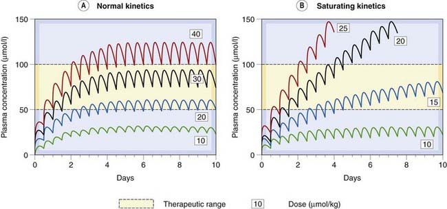
Fig. 10.9 Comparison of non-saturating and saturating kinetics for drugs given orally every 12 h.
[A] The curves showing an imaginary drug, similar to the antiepileptic drug phenytoin at the lowest dose, but with linear kinetics. The steady-state plasma concentration is reached within a few days, and is directly proportional to dose. [B] Curves for saturating kinetics calculated from the known pharmacokinetic parameters of phenytoin (see Ch. 44). Note that no steady state is reached with higher doses of phenytoin, and that a small increment in dose results after a time in a disproportionately large effect on plasma concentration.
(Curves were calculated with the Sympak pharmacokinetic modelling program written by Dr J G Blackman, University of Otago.)
Clinical applications of pharmacokinetics are summarised in the clinical box.
Uses of pharmacokinetics 
Population Pharmacokinetics
In some situations, for example when the drug is intended for use in chronically ill children, it is desirable to obtain pharmacokinetic data in a patient population rather than in healthy adult volunteers. Such studies are inevitably constrained and samples for drug analysis are often obtained opportunistically during clinical care, with limitations as to quality of the data and only sparse data collected from each patient. Population pharmacokinetics addresses how best to analyse such data. Various approaches that have been used, including fitting data from all subjects as if there were no kinetic differences between individuals, and fitting each individual’s data separately and then combining the individual parameter estimates, have obvious shortcomings. A better method is to use non-linear mixed effects modelling (NONMEM). The statistical technicalities are considerable and beyond the scope of this chapter: the interested reader is referred to Sheiner et al. (1997); and, for NONMEM software user guides, to Beale & Sheiner (1989).
Limitations of Pharmacokinetics
Some limitations of the pharmacokinetic approach will be obvious from the above account, such as the proliferation of parameters in even quite conceptually simple models. Here we comment on two assumptions that underpin the idea that by relating response to a drug to its plasma concentration we reduce variability by accounting for pharmacokinetic variation—that is, variation in absorption, distribution, metabolism and excretion:
While the first of these assumptions is very plausible in the case of a drug working on a target in the circulating blood (e.g. a fibrinolytic drug working on fibrinogen) and reasonably plausible for a drug working on an enzyme, ion channel or G-protein-coupled or kinase-linked receptor located in the cell membrane, it is less likely in the case of a nuclear receptor or when the target cells are protected by the blood–brain barrier. In the latter case it is not perhaps surprising that, despite considerable efforts, it has never proved clinically useful to measure plasma concentrations of antidepressant or antipsychotic drugs, where there are, in addition, complex metabolic pathways with numerous active metabolites. It is, if anything, surprising that the approach does as well as it does in the case of some other centrally acting drugs, notably antiepileptics and lithium.
The second assumption is untrue in the case of drugs that form a stable covalent attachment with their target, and so produce an effect that outlives their presence in solution. Examples include the antiplatelet effects of aspirin and clopidogrel (Ch. 24) and the effect of some monoamine oxidase inhibitors (Ch. 46). In other cases, drugs in therapeutic use act only after delay (e.g. antidepressants, Ch. 46), or gradually induce tolerance (e.g. opioids, Ch. 41) or physiological adaptations (e.g. corticosteroids, Ch. 32) which alter the relation between concentration and drug effect in a time-dependent manner.
Pharmacokinetics 
References and Further Reading
Atkinson A.J., Daniels C.E., Dedrick R.L., et al, editors. Principles of clinical pharmacology. London: Academic Press, 2002. (Section on pharmacokinetics includes the application of Laplace transformations, effects of disease, compartmental versus non-compartmental approaches, population pharmacokinetics, drug metabolism and transport)
Birkett D.J. Pharmacokinetics made easy (revised), 2nd edn. Sydney: McGraw-Hill Australia; 2002. (Excellent slim volume that lives up to the promise of its title)
Jambhekar S.S., Breen P.J. Basic pharmacokinetics. London: Pharmaceutical Press; 2009. (Basic textbook)
Beale S.L., Sheiner L.B. NONMEM user’s guides. University of California, San Francisco: NONMEM Project Group; 1989.
Rowland, M., Tozer, T.N., 2010. Clinical pharmacokinetics and pharmacodynamics. Concepts and applications. Wolters Kluwer/Lippincott Williams & Wilkins, Baltimore. Online simulations by H Derendorf and G Hochhaus. (Excellent text; emphasises clinical applications)
Sheiner L.B., Rosenberg B., Marethe V.V. Estimation of population characteristics of pharmacokinetic parameters from routine clinical data. J. Pharmacokinet. Biopharm.. 1997;5:445-479.
1Clinical pharmacology became at one time so associated with the measurement of drugs in urine that the canard had it that clinical pharmacologists were the new alchemists—they turned urine into airline tickets …
2Important because dose-related adverse effects often occur around Cmax.
3For example, doses used in experimental animals often need to be much greater than those in humans (on a ‘per unit body weight’ basis), because drug metabolism is commonly much more rapid in rodents.
4The area is obtained by integrating from time = 0 to time = ∞, and is designated AUC0–∞. The area under the curve has units of time—on the abscissa—multiplied by concentration (mass/volume)—on the ordinate; so CL = Q/AUC0–∞ has units of volume/time as it should.